Spatial Temporal Sediment Hydrodynamics and Nutrient Loads in Nyanza Gulf, Characterizing Variation in Water Quality

ISSN Online: 2331-4249 ISSN Print: 2331-4222

DOI: 10.4236/wjet.2018.62B009 May 22, 2018 98 World Journal of Engineering and Technology

Spatial-Temporal Sediment Hydrodynamics

and Nutrient Loads in Nyanza Gulf,

Characterizing Variation in Water Quality

Angalika W. S. Misigo, Seiji Suzuki

Department of Advanced Engineering, Nagasaki University, Nagasaki City, Japan

Abstract

Accelerated aging and eutrophication of water resources is a world menace attributed to influx of nutrient rich sediment from its catchment, resulting in poor water quality and shifts in ecological dynamism. Nyanza Gulf is a para-mount source of livelihood, portable water, and of service to the rich biodi-versity making it indispensable to the entire Lake Victoria watershed ecosys-tem. This water resource has been deteriorating over the past decades as a consequent of anthropogenic socio-economical activities. This has effectuated an increase in phytoplankton and hydrophyte colonies. The objective of this study was to track the quality and quantity of sediment inundation into the gulf considering the catchment micro-basins processes and influence of hu-man socio-economical activities. Using Quantum Geographic Information System (QGIS) as an interface to Soil and Water Assessment Tool (SWAT) with input of satellite digital elevation model (DEM), local rainfall, soil and land use data sets were utilized to determine the daily variability in sediment and nutrient loads from five major river basins. The SWAT model was suc-cessfully calibrated, and the performance validated with observed hydrological and water quality data. The model achieved identification of seasonal water quality budget filling in knowledge gaps about the catchment. River Nyando, Sondu-Miriu, Awach-Kibuon, Awach-Tende and Kibos discharge sediment loads of 3.91, 1.6, 1.18, 1.06 and 0.78 tons/ha respectively. Total suspended solids (TSS) concentration of up to 578mg/L on average daily is discharged by River Awach-Kibuon. This was associated with intense agricultural activities (>54% of the entire basin) on steep slopes (average 12.97) with Acrisols (15%of the basin) soils that is prone erosion. Poorly managed range-bush land that covers about 10% of this basin also contribute significantly to the TSS yield. River Kibos discharge least TSS concentration of 144.43 mg/L in com-parison with other rivers mainly due gentle slope falling into a plain, low

How to cite this paper: Misigo, A.W.S. and Suzuki, S. (2018) Spatial-Temporal Sediment Hydrodynamics and Nutrient Loads in Nyanza Gulf, Characterizing Variation in Water Quality. World Journal of Engineer-ing and Technology, 6, 98-115.

https://doi.org/10.4236/wjet.2018.62B009

DOI: 10.4236/wjet.2018.62B009 99 World Journal of Engineering and Technology

erodible Cambisols (covers 20% of the basin) and Ferralsols (10%) as well as Nanga forest effect at its exit. River Awach-Tende and Awach-Kibuon on av-erage discharge 1.67 mg/L and 1.58 mg/L respectively of Total Nitrogen (TN) daily. This was linked to intensive farming on poorly managed dominant Phaeozems and Acrisols that are susceptible to leaching. River Sondu-Miriu is the least contributor with a daily average of 1.1101 mg/L dominated with low leached Nitisols. The bay receives highest Total Phosphorus (TP) loads from River Nyando with daily average of 0.3699 mg/L alluded to high biomass production in the basin and Sondu-Miriu least with 0.0288 mg/L. The fluctua-tion of nutrients and sediment fluxes correlated positively with rainfall events. The long rainfall season with average regular storm events in March to June yield highest monthly loads as compared to short rainfall season (September to November) with isolated intense storm events over a shorter time. The study depicted poor water quality discharged into the gulf throughout the year by the 5 major basins to be above average of conventional ecological healthy basins.

Keywords

Micro-Basin, Spatial, Sediment, Nutrient, SWAT, Anthropogenic

1. Introduction

Nyanza (also known as Winam or Kavirondo) gulf forms a cardinal part of larg-er Lake Victoria basin ecosystem that has been degrading at an alarming rate. Signs of degradation of its water resource were first visible in early 1980s [1]. Consequences of this eutrophication have been seasonal occurrence of algal bloom and intensive proliferation of water hyacinths which dates to 1990 [2] [3]. The weed colonies have a huge threat to the productivity of the gulf negatively affecting socioeconomic wellbeing of the population that depends on it for live-lihood. Rapid urbanization along the lake shores and poor land use management under intensive farming have negatively impacted the gulf. Influx of nutrient rich sediment into the lake has increased from both diffuse and point-sources exerting considerable negative effect particularly on the near-shore regions [4] [5]. Between January and March 2004, the persistence of massive phytoplankton blooms in the Nyanza Gulf resulted in a temporary shutdown of the drinking water supply from the lake [6].

Nyanza Gulf has an area of 1400 km2_{, mean depth 7 m, max. depth 30 m and a}

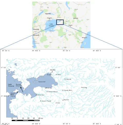
DOI: 10.4236/wjet.2018.62B009 100 World Journal of Engineering and Technology Figure 1. Nyanza Gulf catchment information.

in-DOI: 10.4236/wjet.2018.62B009 101 World Journal of Engineering and Technology

crease of atmospheric deposition remains disputed [3].

Spatial temporal estimation of sediment and nutrient loads is of crucial inter-est for a good assessment of water pollution of such vital water resource in iden-tification and mitigation of water quality and biodiversity [11]. Assessing runoff, soil and nutrient loss in a catchment is important for investigation of soil ero-sion hazards, aquatic shifts and for determining suitable land uses and soil con-servation measures. Such information would be key in optimizing benefit from the use of the land whilst minimizing the negative impacts of land degradation. Physical based SWAT model [12] was developed for analyzing effects of naturo-genic process and anthroponaturo-genic activities on a water resource. The tool quanti-fies the sediment loss in space and time basing on runoff, soil characteristics, land use and slope to predict water quality, sediment yield and pollution loading in the catchment. SWAT model can be taken as a potential tool for simulation of the hydrology of gauged/ungauged watershed in mountainous areas to address the issues related to water quality and evaluate best watershed management practices [13]. Spatial temporal quantification of the water quality parameters in Nyanza bay was studied by application of this promising physical based distri-buted SWAT model interfaced in QGIS [12] [14] [15]. The objective was to de-termine daily discharge of the five (5) major rivers, sediments and nutrients loading to fill in the knowledge gap of understanding the influence of major ba-sins on the water quality in Nyanza gulf (Calibration period 2005-2014 and Va-lidation period 2014-2015).

2. Methodology

2.1. Study Area

Nyanza gulf is in Western Kenya whose watershed lies between 0.25N - 1.00S la-titudes and 34.0E - 36.0E longitudes as shown in Figure 1. It covers an

approx-imate total drainage area of 12,300 km2_{. The Rivers originate from East and}

DOI: 10.4236/wjet.2018.62B009 102 World Journal of Engineering and Technology

susceptible to leaching and Acrisols that are prone to erosion. The fishing indus-try and favorable weather condition have catalyzed rapid urbanization extending to the shore of the lake and uncontrolled farming practices encroaching riparian zones.

2.2. Data Acquisition

The region is covered with three weather stations but only two (2) at Kisii (−00667, +034783) and Kisumu Airport (−00100, +034750) were utilized. Keri-cho (−00367, +035350) station had a lot of inconsistence data. Daily climate data (rainfall, maximum and minimum temperatures, relative humidity and solar radiation was used as model input and monthly data for the Weather Generator (WGN) Parameters. There are no hydrometric stations in this region. Local

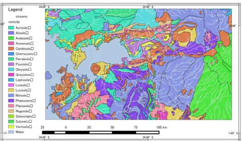
de-tailed Soil data map derived from KENSOTER for studiesof carbon stocks [16]

was used. The soil data (Figure 2) contains detailed information of the 2-soil depth: top soil (0 - 30 cm) and subsoil (30 - 100 cm). Land use statistics was ob-tained from World resource institute-WRI (Figure 3). It contains different classes; Agricultural land use (cereals, sugar, paddy rice/sugar under irrigation, perennial crops like tea), forests (Protected forest, evergreen, deciduous and mixed), Wetland and urban residential. Agriculture is dominant in the region covering more than 60% of the total land use. Crop management was scheduled as; long season I (January-Land preparation, March-planting and fertilization, August-harvesting) and Short Season II (September-land preparation, Octo-ber-planting and fertilization, December harvesting). Digital Elevation model

DOI: 10.4236/wjet.2018.62B009 103 World Journal of Engineering and Technology Figure 3. Detailed map of Land uses in the modeled river basins (COFF = TEA).

(DEM) was derived from Shuttle Radar Topography Mission (SRTM) at 30 m resolution.

2.3. SWAT Model

SWAT is a river or watershed, spatial model developed to predict the impact of land management practices on water, sediment hydrodynamics, and agricultural chemical yields in large complex watersheds with varying soils, land use, man-agement conditions and weather conditions. The model consists of the following main components: Weather, hydrology, plant growth, nutrients (Nitrogen and Phosphorous based), pesticide, bacteria and land management-SWAT version 2012 [17]. The Model is run in QGIS interface enabling integration of spatial distributed characteristics of the watershed into calculations.

DOI: 10.4236/wjet.2018.62B009 104 World Journal of Engineering and Technology

route channel in each sub-basin [19]. These hydrologic processes are based on infiltration, percolation, evaporation, plant uptake, lateral flows and groundwa-ter flows including snowfall and snowmelt [14]. Sediment yield is estimated based on Modified Universal Soil Loss Equation (MUSLE) which factors in the surface runoff volume, the peak runoff rate, the area of the HRU, the Universal Soil Loss Equation (USLE) soil erodibility factor, the USLE cover and manage-ment factor, the USLE support practice factor, the USLE topographic factor, and a coarse fragment factor. On other hand routing phase defines movement of wa-ter, sediments and nutrient loads from each channel network to the outlet. Channel transmission losses, evaporation, return flow etc., are adjusted for esti-mation of outflow from a channel which is predicted by the Muskingum method [20]. The hydrological balance is simulated by SWAT model according to the equation below [21].

1( )

t

t o day surf a seep gw i

SW SW R Q E W Q

=

= +

∑

where: SWt is the final soil water content (mm); SW0 is the initial soil water

con-tent on day i (mm); Rday is the amount of precipitation on day i (mm); Qsurfis the

amount of surface runoff on day i (mm); Eais the amount of evapotranspiration

(ET) on day i (mm); Wseep is the amount of water entering the vadose zone from

the soil profile on day i (mm); Qgw is the amount of return flow on day i (mm).

2.4. Calibration and Uncertainty Analysis

SWAT-Calibration Uncertainty Programs version 2012 (SWAT-CUP) was uti-lized for Calibration/validation, uncertainty and sensitivity analysis of the mod-el. Investigation of sensitivity and uncertainty in stream flow and sediment con-centration was done by Sequential Uncertainty fitting (SUFI-2) algorithm. Sev-eral objective functions were used to gauge model performance by: coefficient of

linear correlation R2_{, Nash-Sutcliffe Efficiency (NSE) and the coefficient of}

per-centage biasness (PBIAS). NSE (Equation (2)) is a normalized statistic that de-termines the relative magnitude of the residual variance in comparison to the measured data variance indicating how well the plot of observed fits the simu-lated data; 1:1 [22] [23]. NSE = 1 is the optimal value, values between 0.0 and 1.0 regarded as acceptable levels of performance of the model, whereas values ≤ 0.0 indicating that mean observed value is a better predictor than simulated value (unacceptable performance of the model).

2 1 2 1 ( ) NSE 1 ( )

n obs sim

i i

i

n obs avg i i X X X X = = − = − −

∑

∑

where obs

i

X is the ith observation for the constituent being evaluated, sim

i

X is

the ith simulated value for the constituent being evaluated, _Xavg _{is the}

aver-age/mean of observed data for the constituent being evaluated, and n is the total

number of observations.

DOI: 10.4236/wjet.2018.62B009 105 World Journal of Engineering and Technology

differences in streamflow/sediment concentration between simulated and meas-ured data for the period of analysis. PBIAS = 0 is optimal indicating unbiased-ness and larger value show more variance between simulated value and observed information. Positive value indicates model overestimation bias, and negative value indicates model underestimation bias.

1

1

( ) 100

PBIAS

( )

n obs sim

i i

i

n obs i i

X X

X =

=

− ∗ =

∑

∑

In this study, model performance for a monthly time and specific day data was judged as satisfactory if NSE > 0.50 and PBIAS = ±25% and graphical analy-sis that reveals a good agreement between predicted and measured hydrographs (R2 _{= 0.6).}

3. Results and Discussion

The capability of a hydrological model to adequately simulate streamflow, sediment and nutrient concentration rely on the precise calibration of its parameters as well as quality input of baseline data sets [24]. Model calibration and validation are indispensable for simulation process in estimating characteristics of a phenomenon that would rather be either impossible or uneconomical for actual study and analysis.

3.1. Model Calibration

The calibration of a conceptual model necessitates setting the input variables to correspond optimally in mimicking measured observations thus representing the reality on of studied phenomenon. It is deliberately carried out with the purpose of defining the values or desirable ranges of the model parameters that depend broadly on the nature and specific properties of the study area. Prelimi-nary analyses, subsequent simulation of databases combination of DEM, preci-pitation, crop and soil, yielded a fair default performance (NSE = 0.0922) before calibration. The impact of soil data set was most significant in the modeling of the basins for discharge and water quality. Calibration of SWAT model in the Nyanza through semi-automated approach (SUFI-2) method was performed over a period of 9 years by comparing the mean monthly measured flow rates (stream flow estimated done by floating method) and sediment concentration to simulated rates. This was performed to the 5 study rivers with monthly mean es-timates of the flow rates and water quality regarding TSS concentration from 2005-2014. The following represents one of the major basins (Figure 4) in Gulf’s catchment during calibration and validation period basing on monthly discharge and concentration of sediments loads.

DOI: 10.4236/wjet.2018.62B009 106 World Journal of Engineering and Technology Figure 4. River Sondu simulated and observed monthly mean flow discharge and Sediment concentration.

Figure 5. Scatter plot of monthly stream flow and Sediment concentration for calibration period (2005-2014).

coefficient of NSE of the order of 0.69 to 0.81 and PBIAS of the order of 9.52 to 21.45. The performance of the model for sediment concentration was within adoptable range with NSE of 0.64 to 0.79 and PBIAS of 9.09 to 19.63. The model

of the largest contributing basin, Sondu River, had coefficient of NSE 0.72, R2 _of

0.82 and PBIAS of 13.32 basing on monthly mean flow rates. The sediment con-centration of the same basin has a coefficient NSE of 0.78, R2 _{of 0.79 and PBIAS of}

DOI: 10.4236/wjet.2018.62B009 107 World Journal of Engineering and Technology

3.2. Model Validation

Validity of a model is gauged on how comparable it is to the actual situation of the study area basing on the series observations done over a defined period. Any calibration procedure of a model should be put necessarily to the control of testing its reliability and performance. Validation of SWAT model of each ba-sin was performed from 2014-2015 (1 year) over the period of calibration (2005-2014) by comparing monthly mean flow rates, specific day sediment and nutrient concentration to measured data (e.g. Figure 6). Sondu Miriu basin. The limnology data was obtained from selective grab samples at the mouth of the rivers and water quality analysis done on specific days during Lake Victoria Comprehensive Research for Development (LAVICORD PROJECT, 2015).

Considering daily simulated results of the model in comparison with the ob-servations, all the modeled river basins showed high performance as indicated below (Table 1). Despite of few observed water quality data for Awach-Tende river, the model response was quite successful indicating both equivalence and trends in the changes (Figure 7 and Table 2). Its probability of biasness was within good range though higher compared to the other models.

The results indicate high inflow of sediments with mean of 578 mg/L, 526 mg/L, 384 mg/L,198 mg/L, and 143 mg/L from Awach-Kibuon, Awach-Tende, Nyando, Sondu Miriu and Kibos respectively as (Figure 8). The highest loads of sediment into the gulf within the study period was found to be in April-May

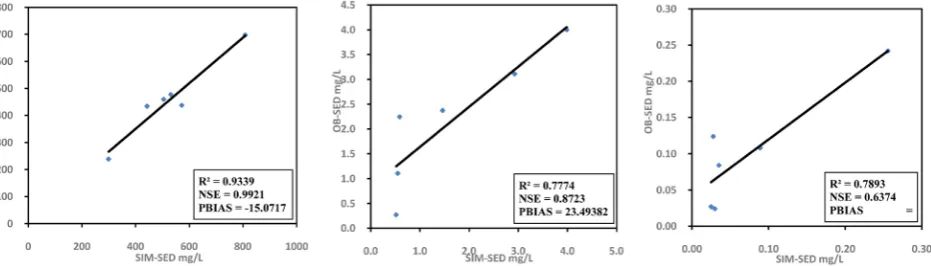
Figure 6. Sondu-Miriu River: scatter plot of specific day sediment and nutrient concentration for validation period (2014-2015).

DOI: 10.4236/wjet.2018.62B009 108 World Journal of Engineering and Technology

Figure 8. Simulated and observed specific day seasonal sediment loads1_.

Table 1. Model performance statistics for the 5-major river Catchment of Nyanza Gulf.

Time step description

Calibration (2005-2014) Validation 2014-2015 (LAVICORD, 2015)

C rit erio n A w ac h-K ibu on So nd u M ir iu N yan do K ibo s A w ac h-Ten de A w ac h-K ibu on So nd u M ir iu N yan do K ibo s A w ac h-Ten de Monthly River Discharge R2 NSE PBIAS (%) 0.7616 0.7334 18.2687 0.8158 0.7243 13.3229 0.7026 0.6905 9.5242 0.7528 0.6971 21.4457 0.7123 0.7268 −10.2543 0.7826 0.8113 11.3781 0.8591 0.7324 15.3546 0.6906 0.7195 11.6472 0.7619 0.7213 17.3465 0.7336 0.7988 −8.5317 Monthly Sediment Concentration R2 NSE PBIAS (%) 0.7894 0. 7285 14.3382 0.7846 0.7821 11.631 0.684 0.7149 −10.0905 0.7455 0.6983 −8.3829 0.7773 −0.6258 12.7829 0.7966 0. 6922 12.3520 0.8133 0.7212 19.631 0.7281 0.7849 −9.0905 0.7568 0.7268 −9.9540 0.8614 0.5415 6.1345

Lack monthly mean data for Nutrient concentration calibration was based on isolated studies (Lake Victoria Environmental

Management Project PHASE I, 1995 and PHASE II, 2008) Validation 2014-2015 (LAVICORD, 2015)

Specific sampled Day Sediment Concentration R

2 NSE PBIAS (%) 0.7840 0.6149 −16.0905 0.6689 0.5119 23.3571 0.7093 0.7027 −24.3322 0.8554 0.7058 11.4173 0.9339 0.9921 −15.0717

Specific sampled Day Total Nitrogen Concentration R

2 NSE PBIAS (%) 0.7554 0.6810 18.0824 0.7760 0.6845 17.9087 0.8126 0.7046 13.6827 0.8618 0.6596 19.9562 0.7774 0.8723 23.49382

Specific sampled Day Total Phosphorous Concentration R

2 NSE PBIAS (%) 0.7847 0.7319 −4.1887 0.8126 0.5939 7.2427 0.7373 0.6258 −6.8782 0.7100 0.7642 15.7204 0.7893 0.6374 24.0044

during long rains followed by October-November during short rain season. Total nitrogen and Phosphorous Loads were substantially high in April – May as modeled in Figure 9 & Figure 10 attributed to high precipitation and agri-cultural activities within the entire catchment.

1_{AWA-KI-River Awach-Kibuon, SO-River Sondu Miriu, NYA-River Nyando, KIB-River Kibos,}

DOI: 10.4236/wjet.2018.62B009 109 World Journal of Engineering and Technology Table 2. Awach-Tende simulated and observed specific day seasonal sediment and nu-trients loads.

DATES SIM-SED _mg/L OB-SED mg/L SM-TN mg/L OB-TN mg/L SIM-TP _mg/L OB-TP mg/L

6/26/2014 299.231 338.541 0.518 0.271 0.028 0.124

9/1/2014 808.648 697.756 2.926 3.111 0.256 0.242

11/4/2014 572.284 437.750 1.463 2.375 0.089 0.108

1/13/2015 442.664 434.254 0.590 2.247 0.035 0.084

3/27/2015 504.941 459.750 3.985 4.002 0.025 0.027

6/25/2015 531.204 477.170 0.550 1.108 0.030 0.024

Figure 9. Simulated and observed specific day seasonal total nitrogen loads.

Figure 10. Simulated and observed specific day seasonal total Phosphorous loads.

3.3. Uncertainty Analysis

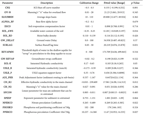
DOI: 10.4236/wjet.2018.62B009 110 World Journal of Engineering and Technology Table 3. Summary of the SWAT model Parameters calibrated on the major river basins in Nyanza gulf catchment.

Parameter Description Calibration Range Fitted value [Range] p-Value

CN2 SCS Run off curve number −0.5 - 0.5 0.155 [−0.199; 0.252] 0.001

OV-N Manning’s’ “n” value for overland flow 0.01 - 28 21.23 [3.061; 29.915] 0.345

SLSUBBSN Average slope basin 10 - 110 49.808 [12.677; 49.924] 0.362

ALPHA_BF Base flow alpha factor −0.2 - 0.1 0.679

ESCO Soil evaporation compensation factor 0.01 - 1 0.898 [0.768; 0.991] 0.714

SOL_AWS Available water content of the soil −0.35 - 0.25 0.120 [−0.0169; 0.197] 0.016

SOL_BD Moist bulky density 0.110 - 0.139 0.116 [0.112; 0.195] 0.426

GW_DELAY Ground water Delay 0.0 - 100 34.938 [0.487; 49.823] 0.37

SURLAG Surface Runoff lag time 0.05 - 30 20.219 [0.076; 23.878] 0.831

REVAPMN Threshold depth of water in the shallow aquifer for _{“revap” or percolation to the deep aquifer to occur} 0 - 500 173.709 [0.636; 499.845] 0.516

GW-REVAP Groundwater revap coefficient −0.02 - 0.2 0.190 [0.021; 0.199 0.522

SOL-K Saturated Hydraulic conductivity 0.17 - 0.65 0.183 [0.18; 0.265] 0.05

USLE_K Saturated hydraulic conductivity (mm/h) −0.173 - 0.59 0.209 [0.08; 0.227] 0.366

USLE_P USLE equation support factor 0.35 – 0.76 0.456 [0.384; 0.6898] 0.021

ADJ_PKR Peak Adjustment factor (sediment routing in sub-basin) 0.537 - 1.167 0.647[0.622;1.134] 0.364 CH_K2 Effective hydraulic conductivity in the main channel −0.010 - 239.609 17.961 [16.98; 114.313] 0.012 CH_N2 Manning’s “n” value for the main channel 0.027 - 0.091 0.051 [0.026; 0.059] 0.286 SPCON Linear parameter for max am sediment that can be _re-entrained 0.005 - 0.011 0.007 [0.00115 - 0.0023] 0.483 SPEXP Exponent parameter for sediment re-entrained 0.753 - 1.151 1.001 [0.825 - 1.09] 0.064

NPERCO Nitrate percolation Coefficient 0.265 - 0.489 0.269 [0.265; 0.385] 0.022

PHOSKD Phosphorus soil partitioning coefficient m3_{/Mg 102 - 200 178 [166; 183] 0.324}

PPERCO Phosphorous percolation Coefficient 10m3_{/Mg 10.237 - 14.368 11.67 [10.953; 14.335] 0.027}

flow, Sediment and nutrient loads of the 5 basins. Based on the 22 selected SWAT parameters, globalized sensitive analysis was used for identifying sensi-tive and important model parameters while holding ALPHA_BF at fixed value. Several iterations and simulations of each basin independently till acceptable

re-sults were realized. Eight (8) parameters i.e.CN2, CH_K2, SOL_AWC, USEL_P,

NPERCO, PPERCO, SOL_K and SPEXP were found to be the most sensitive for the gulf catchment in entirety. The performance of the SWAT model for the 5 basins was good during calibration with NSE > 70, thus consistency in the data sets utilized.

3.4. Sediments and Nutrient Yield

The model results demonstrate responsiveness between the precipitation and river discharge with similar pattern over the entire study period. Table 4

indi-cates an average total stream discharge of 87.629 m3_{/s water from the five major}

to-DOI: 10.4236/wjet.2018.62B009 111 World Journal of Engineering and Technology

pography and high rainfall in Sondu Miriu explains the significant high dis-charge when compared to Nyando that is largely a plateau.

3.4.2. Spatial Sediment and Nutrients Yield

SWAT model simulates loss of sediment transport in a catchment basing on MUSLE equation relating runoff, soil characteristics, land use, topography and land management practices. Quantity of sediments eroded and conveyed to the hydrographic network at each spatial unit can be adequately estimated with SWAT model [21]. Part of estimated soil eroded particles, flow into the stream leading to increase in water turbidity. Seasonal sediment concentration (Figure 11) in water discharged to Gulf was temporal attributed to changes precipitation and localized factors in individual HRUs.

Table 4. Annual rainfall and mean river discharge.

Name of the river

Annual rainfall (mm)

OB-Mean discharge (m3_/s)

SIM-Mean river discharge (m3_/s)

Size of the Catchment

(km2₎

Sondu-Miriu 1573 44.92 44.240 3448.542

Nyando 1327 20.37 20.237 3597.808

Awach-Tende 1573 10.54 11.366 686.426

Awach-Kibuon 1573 8.18 8.464 549.149

Kibos 1327 4.67 4.322 560.745

DOI: 10.4236/wjet.2018.62B009 112 World Journal of Engineering and Technology

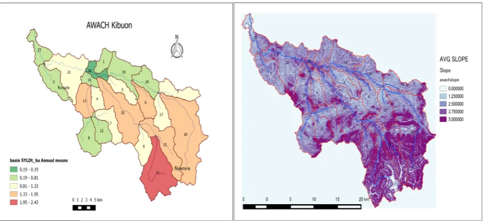
Spatially, Agricultural activities on steep slopes e.g. cereal and tea farming in Kisii and Nyamira resulted into substantial sediments loss in the Awach-Kibuon basin (Figure 12 basins 6, 16, 11, 15 and 18). Phaeozems (58%), Nitisols (25%) and Acrisols (15%) are the most abundant soil in this basin. Acrisols are easily eroded while Poor land management Phaeozems and Nitisols on steep slopes showed proneness to erosion as indicated by high sediments yield from the range-bush land use (Awach-Kibuon basins 21 & 13) source of sediments. Water quality at the mouth of Kibos River had less sediment concentration that was at-tributed to its low average slope and riparian effect of the forest at Nanga area.

Nutrient concentrations in water resources are indispensable of sediment transport [26]. Nyando River showed notably high phosphorous concentrations; majorly organic phosphorus probably from the forest and resultant biomass in the catchment (sugar, rice and other cereals refuse). Substantial nitrogen con-centration from Awach-Tende and Awach-Kibuon (dominated by Phaeozems and Acrisols that are intensively leached in wet seasons) can be linked to intense use of nitrogen fertilizers in Kisii highlands for cereal and Tea farming. Influ-ence of Urban activities led to the high Nitrogen concentration in the Kibos ba-sin. Discharge from the 5-basins showed poor water quality throughout the year and high concentration of nutrients (Table 5).

Figure 12. Spatial sediment yield in Awach-Kibuon River and average slope influence.

Table 5. Simulated water quality and sediment loads.

RIVER AREA ha TSS mg/L TN mg/L TP mg/L SED LOAD ton/ha/yr

Awach-Kibuon 54,914.9 577.59 1.5431 0.3089 1.08

Awach-Tende 68,642.6 526.50 1.6700 0.0823 0.96

Nyando 359,780.8 384.43 1.1687 0.3699 4.07

Kibos 56,074.5 143.02 1.5561 0.1070 0.8

DOI: 10.4236/wjet.2018.62B009 113 World Journal of Engineering and Technology

4. Conclusion

Spatial-temporal SWAT model used in this study was successfully calibrated and validated for the 5 major basins generating adequate results on seasonal varia-tion in river water quality. Spatial approach of these models integrates hydrolo-gy, vegetation, erosion and nutrient dynamics to obtain hydrological functioning of each mesoscale sub-basins units process, production and transfer of sedi-ments and nutrients. The model herein plays a vital role in assessing different human activities in the catchment and thereafter effects on water resource with respect to time and space. For instance, intense farming on the Kisii highlands dominated with highly erosion prone Acrisols, yield highest annual sediments of up to 2.4 tons/ha while Plains dominated cambisoils resulted to lowest annual sediment yield of up to 0.089 tons/ha. Cereal, Tea farming and poor maintained range-bushland use were main contributors to poor water quality in the five-major rivers. Effect of poor urban management and disposal can be linked to high Nitrogen concentrations that couldn’t be precisely modeled in Kibos River basin. The study depicted poor water quality discharged into the gulf by the 5 major basins to be above average of conventional ecological healthy basins (TP of 0.01 - 0.04 mg/L, TN of 0.1 - 0.5 mg/L, TSS of 2 - 5 mg/L). The model ap-plicability in the five river basins was adequate for performance of monthly time and daily step satisfied NSE > 0.50, PBIAS = ±25% and graphical analysis that revealed a good agreement between predicted and measured hydrographs. Thus, can be used to evaluate impact of natural and anthropogenic activities in the catchment on water quality discharge. Detailed spatial-temporal information can be utilized in locating issues and applying mitigation for soil loss consequently improving quality of water discharged in the Gulf. Recommendation for further point pollution, offshore activities and ecohydrological studies within the gulf need to be carried out basing on daily imports of the materials into gulf to de-termine effects of each part of the catchment on deterioration of water quality implicated by appearance of seasonal algal bloom.

Acknowledgements

The authors wish to thank JICA (Japanese International Cooperation Agency) for their support through ABE-Initiative Scholarship and Nagasaki University fraternity for provision of facilities and resource to make this study possible.

Conflicts of Interest

The author declares no conflict of interest.

References

[1] Ochumba, P.B.O. and Kibaara, D.I. (1989) Observations on Blue-Green Algal

Blooms in the Open Waters of Lake Victoria, Kenya. Afr. J. Ecol., 27, 23-34.

https://doi.org/10.1111/j.1365-2028.1989.tb00925.x

DOI: 10.4236/wjet.2018.62B009 114 World Journal of Engineering and Technology

Water Hyacinth in Lake Victoria and the Kagera River Basin, 1989-2001. J. Aquat.

Plant Manag., 42, 73-84.

[3] MCI (2009) An Overview of the Main Environmental Issues Affecting Kisumu and

Lake Victoria’s Winam Gulf.

[4] Verschuren, D., Johnson, T.C., Kling, H.J., Edgington, D.N., Leavitt, P.R., Brown,

E.T., Talbot, M.R. and Hecky, R.E. (2002) History and Timing of Human Impact on

Lake Victoria, East Africa. Proc. R. Soc. B Biol. Sci., 269, 289-294.

https://doi.org/10.1098/rspb.2001.1850

[5] Hecky, R.E., Mugidde, R., Ramlal, P.S., Talbot, M.R. and Kling, G.W. (2010)

Mul-tiple Stressors Cause Rapid Ecosystem Change in Lake Victoria. Freshw. Biol., 55,

19-42. https://doi.org/10.1111/j.1365-2427.2009.02374.x

[6] Sitoki, L., Kurmayer, R. and Rott, E. (2012) Spatial Variation of Phytoplankton

Composition, Biovolume, and Resulting Microcystin Concentrations in the Nyanza

Gulf (Lake Victoria, Kenya). Hydrobiologia, 691, 109-122.

https://doi.org/10.1007/s10750-012-1062-8

[7] Alexander, R., Antenucci, J.P., Attwater, G., Ewing, T., Feaver, S., Imberger, J.,

Khi-sa, P., Lam, C., Njuguna, H. and Shimizu, K. (2006) Management Implications of the Physical Limnological Studies of Rusinga Channel and Winam Gulf in Lake

Victoria, Victoria. 63-68. http://www.oceandocs.org/handle/1834/2327

[8] Gikuma-Njuru, P., Hecky, R.E., Guildford, S.J. andMacintyre, S. (2013) Spatial

Va-riability of Nutrient Concentrations, Fluxes, and Ecosystem Metabolism in Nyanza

Gulf and Rusinga Channel, Lake Uictoria (East Africa). Limnol. Oceanogr, 58,

774-789. https://doi.org/10.4319/lo.2013.58.3.0774

[9] Guya, F.J. (2013) Bioavailability of Particle-Associated Nutrients as Affected by

In-ternal Regeneration Processes in the Nyanza Gulf Region of Lake Victoria, Lakes.

Reserv. Res. Manag, 18, 129-143. https://doi.org/10.1111/lre.12031

[10]Gikuma Njuru, P. (2008) Physical and Biogeochemical Gradients and Exchange

Processes in Nyanza Gulf and Main Lake Victoria ( East Africa ) by.

[11]Quilbé, R., Rousseau, A.N., Duchemin, M., Poulin, A., Gangbazo, G. and Villeneuve,

J.P. (2006) Selecting a Calculation Method to Estimate Sediment and Nutrient Loads

in Streams: Application to the Beaurivage River (Québec, Canada). J. Hydrol., 326,

295-310. https://doi.org/10.1016/j.jhydrol.2005.11.008

[12]Gassman, P.P.W., Reyes, M.M.R., Green, C.C.H. and Arnold, J.J.G. (2007) The Soil

and Water Assessment Tool: Historical Development, Applications, and Future

Re-search Directions. Trans. ASAE, 50, 1211-1250. https://doi.org/10.13031/2013.23637

[13]Shawul, A.A., Alamirew, T. and Dinka, M.O. (2013) Calibration and Validation of

SWAT Model and Estimation of Water Balance Components of Shaya Mountainous

Watershed, Southeastern Ethiopia. Hydrol. Earth Syst. Sci. Discuss, 10, 13955-13978.

https://doi.org/10.5194/hessd-10-13955-2013

[14]Neitsch, S.L., Arnold, J.G., Kiniry, J.R. and Williams, J.R. (2009) Soil & Water

As-sessment Tool Theoretical Documentation.

[15]Gassman, P.W., Reyes, M.R., Green, C.H. and Arnold, J.G. (2007) The Soil and

Wa-ter Assessment Tool: Historical Development, Applications, and Future Research

Directions. Trans. ASABE, 50, 1211-1250. https://doi.org/10.13031/2013.23637

[16]Batjes, N.H. and Gicheru, P. (2004) Soil Data Derived from SOTER for Studies of

Carbon Stocks and Change in Kenya. ISRIC World Soil Inf. Rep., 37.

http://www.isric.org/isric/webdocs/Docs/ISRIC_Report_2004_01.pdf

DOI: 10.4236/wjet.2018.62B009 115 World Journal of Engineering and Technology (2012) Soil and Water Assessment Tool “SWAT” Input/Output Documentation Version 2012.

[18]Patel, D.P. and Srivastava, P.K. (2013) Flood Hazards Mitigation Analysis Using

Remote Sensing and GIS: Correspondence with Town Planning Scheme. Water

Re-sour. Manag., 27, 2353-2368. https://doi.org/10.1007/s11269-013-0291-6

[19]Rafiei, E.A., Kappas, M., Hoang Khanh Nguyen, L. and Renchin, T. (2017)

Hydro-logical Modeling in an Ungauged Basin of Central Vietnam Using SWAT Model.

Hydrol. Earth Syst. Sci., 4, 2-17.

[20]Baymani-Nezhad, M. and Han, D. Hydrological Modeling Using Effective Rainfall

Routed by the Muskingum method (ERM). J. Hydroinformatics.

[21]Arnold, J.G., Kiniry, J.R., Srinivasan, R., Williams, J.R., Haney, E.B. and Neitsch, S.L.

(2013) Soil & Water Assessment Tool: Input/Output Documentation. Version 2012.

[22]Nash, J.E. and Sutcliffe, J.V. (1970) River Flow Forecasting through Conceptual

Models Part I: A Discussion of Principles. J. Hydrol., 10, 282-290.

https://doi.org/10.1016/0022-1694(70)90255-6

[23]Moriasi, D.N., Arnold, J.G., Van Liew, M.W., Bingner, R.L., Harmel, R.D. and Veith,

T.L. (2007) Model Evaluation Guidelines for Systematic Quantification of Accuracy

in Watershed Simulations. Trans. ASABE, 50, 885-900.

https://doi.org/10.13031/2013.23153

[24]Xu, Z.X, Pang, J.P., Liu, C.M. and Li, J.Y. (2009) Assessment of Runoff and

Sedi-ment Yield in the Miyun Reservoir CatchSedi-ment by Using SWAT Model. Hydrol.

Process, 23, 3619-3630. https://doi.org/10.1002/hyp.7475

[25]Niraula, R., Meixner, T. and Norman, L.M. (2015) Determining the Importance of

Model Calibration for Forecasting Absolute/Relative Changes in Streamflow from

LULC and Climate Changes. J. Hydrol., 522, 439-451.

https://doi.org/10.1016/j.jhydrol.2015.01.007

[26]Somura, H., Takeda, I., Arnold, J.G., Mori, Y., Jeong, J., Kannan, N. and Hoffman,

D. (2012) Impact of Suspended Sediment and Nutrient Loading from Land Uses

against Water Quality in the Hii River Basin. Japan, J. Hydrol., 450-451, 25-35.