Prediction Based on Generalized Order Statistics from a Mixture of Rayleigh Distributions Using MCMC Algorithm

(1)

Prediction Based on Generalized Order Statistics from a

Mixture of Rayleigh Distributions Using

MCMC Algorithm

Tahani A. Abushal1_{, Areej M. Al-Zaydi}2

1_{Department of Mathematics, Umm Al-Qura University, Makkah Al-Mukarramah, KSA} 2_{Department of Mathematics, Taif University, Taif, KSA}

Email: tabushal@yahoo.com, aree.m.z@hotmail.com

Received May 15, 2012; revised June 16, 2012; accepted June 30, 2012

ABSTRACT

This article considers the problem in obtaining the maximum likelihood prediction (point and interval) and Bayesian prediction (point and interval) for a future observation from mixture of two Rayleigh (MTR) distributions based on generalized order statistics (GOS). We consider one-sample and two-sample prediction schemes using the Markov chain Monte Carlo (MCMC) algorithm. The conjugate prior is used to carry out the Bayesian analysis. The results are specialized to upper record values. Numerical example is presented in the methods proposed in this paper.

Keywords: Mixture Distributions; Rayleigh Distribution; Generalized Order Statistics; Record Values; MCMC

1. Introduction

The concept of generalized order statistics GOS was introduced by [1] as random variables having certain joint density function, which includes as a special case the joint density functions of many models of ordered random variables, such as ordinary order statistics, ordinary record values, progressive Type-II censored order statistics and sequential order statistics, among others. The GOS have been considered extensively by many authors, some of them are [2-18].

In life testing, reliability and quality control problems, mixed failure populations are sometimes encountered. Mixture distributions comprise a finite or infinite number of components, possibly of different distributional types, that can describe different features of data. In recent years, the finite mixture of life distributions have to be of con- siderable interest in terms of their practical applications in a variety of disciplines such as physics, biology, geology, medicine, engineering and economics, among others. Some of the most important references that discussed different types of mixtures of distributions are [19-25].

Let the random variable follows Rayleigh lifetime model, its probability density function (PDF), cumulative distribution function (CDF) and reliability function (RF) are given below:

T





0, 0 ,

t 

  





0, 0 , t 

 

2

, t R t e

 

2 , h t te

 

2

1 t ,

H t  e

2

t



 ₍₁₎

(2)

(3) Also, the hazard rate function (HRF)

 

t 2 ,t (4)

  

 

   

where  . h . R . .

The cumulative distribution function (CDF), denoted by H t

 

, of a finite mixture of k components, denoted by Hj

 

t ,j1, , k

 

1

,

k j j j

is given by

H t p H t





1, ,

j k

(5)

where, for   p 0

1. k

p

the mixing proportions j

and



j₁ j k2

p p 1 p

The case of , in (5), is practical importance and so, we shall restrict our study to this case. In such case, the population consist of two sub-populations, mixed with proportions ₁ and ₂  ₁. In this paper, the components are assumed to be Rayleigh distribution whose PDF, CDF, RF and HRF are given, respectively, by

 

1 1

 

2 2

 

h t p h t p h t (6)

 

1 1

 

2 2

 

,

H t  p H t p H t (7)

 

1 1

 

2 2

 

,

R t p R t p R t (8)

 

t h t

   

R t ,

 

1, 2

j

(2)

T. A. ABUSHAL, A. M. AL-ZAYDI 357

0 1

that  pj ,p1p21 and j

 

,Hj

   

t ,R tj are

given from (1)-(3) after using h t

j

 instead of.

Several authors have predicted future order statistics and records from homogeneous and heterogeneous populations that can be represented by single component distribution and finite mixtures of distributions, respectively. For more details, see [9,10,26].

Recently, a few of authors utilized the GOS’s in Bayes- ian inference. Such authors are [7-9,18]. Bayesian infer- ences based on finite mixture distribution have been discussed by several authors such that: [23,24,27-33].

For Bayesian approach, the performance depends on the form of the prior distribution and the loss function assumed. A wide variety of loss functions have been de- veloped in the literature to describe various types of loss structures. The balanced loss function was suggested by [34]. [35] introduced an extended class of the balanced loss function of the form

 







0

 

  

,

, 1

 

 

0 , ,

L _

 



,



,

           

  

 

 

.



 



,

 (10)

where is a suitable positive weight function and



 

 

 

is an arbitrary loss function when estimate- ing   by  . The parameter 0 is a chosen prior

estimator of 

 



0

, obtained for instance from the crite- rion of maximum likelihood (ML), least squares or unbi- asedness among others. They give a general Bayesian connection between the case of  0 and  

, 0,

k k

r where 0 1.





  

, ,

m m n

Suppose thatT1; , ,n m k ,T2; , ,n m k , , Tr n m; , ,

1_, _{, ,}

r

r R m m

 

   

1 r

t t

    



R



1 1 1 r1 are the first

(out of ) GOS drawn from the mixture of two Ray- leigh MTR distribution. The likelihood function (LF) is

given in [1], for by

m

 

1

 

1

i

m r

r i R ti h t 



 _ _ 

 

 









tr



, 

1 1

,

.

r

r i i i

n i

C k

M _ i

  

  

  

 





 

i

R t

 

1

 

,

r

i tr h tr

   

1

0,

i

n i M 



i

p

1



, ,



L  t C R

(11)

where , is the parameter space,

and

t t 

1 

(12)

where and are given, respectively, by (5) and (7).



h t

The purpose of this paper is to obtained the maximum likelihood prediction (point and interval) and the Bayes prediction (point and interval) in the case of one-sample scheme and two-sample scheme. The point predictors are obtained based on balanced square error loss (BSEL)

function and the balanced LINEX (BLINEX) loss function. We used ML to estimate the parameters, and

j

 of the MTR distribution based on GOS. The conjugate prior is assumed to carry out the Bayesian analysis. The results are specialized to the upper record values. The rest of the article is organized as follows. Section 2 deals with the derivation of the maximum likelihood estimators of the involved parameters. Sections 3 and 4, deals with studying the maximum likelihood (point and interval) and the Bayes prediction (point and interval) in the case of one-sample scheme and two-sample scheme. In Section 5, the numerical computations results are presented and the concluding remarks.

2. Maximum Likelihood Estimation (MLE)

Substituting (6), (7) in (11), the LF takes the form

 

1

1 1 2 2 1

1 1 1 2 2 .

i

r

m r

i i

i r

i i

i

r r

L t p R t p R t

p h t p h t

p R t p R t 

 

 



 

 _  _

  

 



 

 



 

(13)

Take the logarithm of (13), we have

 





 

1

1 1 2 2

1

1 1 2 2

1

1 1 2 2

ln ln

+ ln

1 ln ,

r

i i i

i r

i i

i

r r r

l L t m p R t p R t

p h t p h t

p R t p R t

 



 



 

  _  _

  

 

  _  _



, 1

p p p p

(14)

where 1 2 

p

. Differentiating (14) with re- spect to the parameters and j and equating to zero gives the following likelihood equations

 

  

  

   

  

  

1

* *

1 1

* *

1

1 0,

1, 2

r r

i i i r r

i i

r

j j i j i i

j r

i j i r j r

i l

m t t t

p l

p t t

m t t

j

   

 



  



 

 



 _ _ _ _ _



 _



   

            



1, 2 j

(15)



where, for

 

_{ }

 

_{ }

 

_{ }

 

_{ }

 

1 2 * 1 2

2 *

2

, ,

1

i i i i

i i

j i i j i

j i j i

i i

j i i

j

h t h t R t R t

t t

h t R t

h t t R t

t t

h t R t

t t

 

 





 

 

 

    

(16)



 

    

 

(3)

p Equations (15) do not yield explicit solutions for and j, and have to be solved numerically to obtain the ML estimates of the three parameters. New- ton-Raphson iteration is employed to solve (15).

1, 2 j

, ,

T T

n

Remark: The parameters of the components are assumed to be distinct, so that the mixture is identifiable. For the concept of identifiability of finite mixtures and examples, see [19,36,37].

3. Prediction in Case of One-Sample Scheme

Based on the informative 1; , ,n m k r n m k; , , GOS’s from

the MTR distribution, for the remaining unobserved future ( r) components, let Ts n m k; , , , s = r + 1, r + 2,,n denote the future lifetime of the _sth_component to fail, 1 s



n r



, the maximum Likelihood prediction (point (MLPP) and interval (MLPI)), Bayesian prediction (point (BPP) and interval (BPI)) can be obtained.

The conditional PDF of Ts Ts n m k; , , given that the components that had already failed is

 ; , ,

r r n m k

T T 

 

_

_

 





 

1

 

*

1

1 1

1

1 1

ln ln

1 !

, 1,

( 1) 1 !

s r

s r

s r r s

k k

s r s

 

1

1 1

, 1,

s r

s r m

r s

s r s

R t

R t R t h t m

 

m s

s r

r k

k t t R t R t

s r

R t R t h t m

C

R t

m s r C

 



 

  

 

 

 

 

 

_ _ _ _  

1 m 

 

 



 

 

 

 

_ _ _ _

 _



  

(17) In the case when , substituting (6) and (7) in (17), the conditional PDF takes the form

 

* 1

1

1 1 2 2 1 1

1 1 2 2

1

1 1 2 2

ln

ln ]

s j

k

s s

r r

s r

s s

k t

p R t p R t p R t

p R t p R t

 

2 2

1 1 2 2 , .

k

r r

s s s r

p R t

p h h t t t





t p



 

 

_  _ _  _



_ _  _



 

 _  _ _

   

 

1 m 

(18)

And in the case when , substituting (6) and (7) in (17), the conditional PDF takes the form

 

*

2 1 1

1 1 2 2

1 1 2

1 1 2 2

s j s

 

1 1 2 2

1 2

1 1

1 1 2 2 , .

s r

s

r r

m

r r

s r m

s s

s s s r

t

t t t



 





  

 

 

 

 



 

  _

   





 



(19)

In the following, we considered two cases: the first is when the mixing proportion p is known and the second is when the two parameters

k t p R t p R

p R t p R

p h t p h

  



 _



 



 and p are assumed to be unknown.

3.1. Prediction When p Is Known

In this section we estimate 1 and 2, assuming that

the mixing proportion, p₁ and p₂ are known.

3.

n

p r

1.1. Maximum Likelihood Prediction

Maximum likelihood predictio can be obtain using (18) and (19) by replacing the shape aramete s 1 and 2

by ˆ₁_{ }ML and ˆ2 ML which is obtained from (15).

1) Interval prediction

The MLPI for any future observation ts, s = r + 1, r + 2, , n can be obtained by

   





   





*

2 s ˆ1ML,ˆ2ML ds

k t   t

 *

1 ˆ1 ˆ2

Pr ts  _v k s ML, L d ,t ms 1,



, 1.

M t

m v

     

 





t

 (20)



A



1 



100% MLPI (L,U) of the futu observ - tion

re a

s

t is given by solving the following two nonlinear equations

 

P )

2

s t

r 1 , Pr ( .

2

s

t L t t  t U t 

        

    (21)

2) Point prediction

The MLPP for any future observation ts, s =

+ 2, , n can be obtained by replacing the shape pa-rameters 1

r + 1, r by ˆ₁_{ }_ML ₂_{ }

and

 2  and ˆ ML

 

 which, obtained from (15)

 



   



   





1 1 2

*

2 1 2

, d , 1,

ˆ _,ˆ _{d ,} ₁

s _v s ML ML s

s ML ML s v

E t k t t m

k t t m

 



* ˆ ˆ

ˆ s ML

t 

.

   

 



(22)

3.1.2. Bayesian Prediction

When the mixing proportion, p is known. Let the parameters j , j1, 2 have a gamma prior distribution with PDF

 

1 1





π , , , 0 .

Γ( )

j j j j

j j j j j j

j

e

   

     



 

  (23)

These are chosen since they are the conjugate priors for the individual parameters. The joint prior density function of  



 1, 2



is given by

 

₁

π ,

 

2 1

1 1 2 2

2 1

π π π ,

j j

j j

j

j e

  

  

   



(24)

 



_

(4)

It then follows, from (13) and (24), that th

ven by



e joint posterior density function is gi

 

2 1 1 *

1 1 1

1 1 2 2

2

π j j j jj

i

j j

m i

t A e

R t p R

  

    











 

1 1

1 1 2 2

1

1 1 2 2

]

r

i i

r

i i

i

r r

p t

p h t p h t

p R t p R t 

 







  

 

_  _



(25)

where

 

1 π d .

A L t



1 _ _ _



(26) The Bayes predictive density functi

 _

on can be obtained using (18), (19) and (25) as follow:

 

* 1 *

1 ₀ 1 2

d , 1,

d ,

s s j

Q t t t k t m

  



  





iction interval, for the future observation

* *

1 ₀ 1

* *

π

π  1. (27)

Bayesian pred

; , , ,

s n m k

T  s r 1,r2, , n can be computed by approximated Q t1

 

st using the MCM

[17,24], using the form

* _{C algorithm, see}

 

1 *

1

* i

s i s

1

,

* _d

s r

j i j s i t k t t

 _



 

(28)

k t Q t t

 _

  



where  is the number of generated parameters and i

j

 , i1, 2,3, , . They are generated from the poste-

rio ) using Gibbs sampler and Me-

1  100% BPI (L, r density function (25 tro

A

polis-Hastings techniques, for more details see [38].



 



U) of the future observation s

t is given by g the following two nonlinear equations

solvin

 

* 1

* 1 _r

i t

d

1 ,

2 d

i s j s i L

i s j s

k t t



 _



 

  

 







(29)

 

* 1

d . 2 d

r

i s j s i U

i s j s i t

k t t

 _



 

 



 

(30)

Numerical methods are generally necessary to solve the above two equ

gi

ations to obtain L and U for a ven .

2) Point prediction

a) BPP for the future observation ts based on BSEL





function can be obtained using

    1  E t t

 

s , (31)

where _{ }

s BS s ML

t  t 

s ML

t is the ML prediction for future obser-

vation

the

s

t which can be obtained using (22) and E t_s t



can be obtained using

 

_Q*

 

_{d .}

1

r

s _t s s s

b) BPP for the future observation

E t t 



t t t t (32)

s

t BLINX

loss functio

based on n can be obtained using

  1ln s ML 



1





s



,

at _at

s BL

t e e t

a

 _

E

 

  __     __

 ₍₃₃₎

where t_{s ML}_{ } is the ML prediction for the vation

future obser- s

t which can be obtained using (22) and



ats t



c

E e an be obtained using





*

 

1 d .

s r

at

s

at

s s

t e Q t t t





(34)

3.2. Prediction When p and θj Are Unknown

W e

E e t  

hen both of the two parameters th mixing proportion j

p and _j,j1, 2, are assumed to be unknown.

3.2.1. Maximum Likelihood Prediction

Maximum likelihood prediction can be obtain using (18) ) by

and (19 replacing the parameters p, ₁ and ₂ by pˆ_{ }_ML,ˆ₁_{ }_ML and ˆ₂_{ }_ML which we obtained using

(15).

The MLPI for any future observation ts, s r 1, r

2, , n can be obtained by



     





     





*

2 ˆ ,ˆ1 ,ˆ2 d , 1.

v

s ML ML ML s

v k t p   t m

 *

1 ˆ ˆ1 ˆ2

Pr ts t k t ps ML , ML , ML d ,t ms



1,

    

  





(35)



A



1 



100% MLPI (L,U) of the future observation ts is given by solving the following two nonline r Equations ( 1).

2) P iction

a 2

oint pred

e observation ,

The MLPP for any futur ts 1, sr r

2, ,n

  can be obtained by replacing p, ₁

the shape pa-rameters  and 2 by pˆ ML,ˆ1 ML and ˆ2 ML

which, obtained from

 

(15).



     



     





*

1 1 2

*

2 1 2

ˆ ˆ

ˆ ˆ , , d , 1,

ˆ ˆ

ˆ , , d , 1.

s s s s

s ML _t ML ML ML

s s ML ML ML s

t

t E t t k t p t m

t k t p t m

 



   





(36)



3.2.2. Bayesian Prediction

(5)

   

   ,



 j, j,



(37) A joint prio

1

1 _{0 .}

Γ j j j j j j

j j j

j j p e                _ _   

r density function of 



p, , ₁ ₂



is

then given by

 

     

 

21

3 2 1 π , , j 1 2

1 2 1

1 1 1

2 2

π π π

π ₁ j _e j j j

         1,p b b j p p p        



j 1   (38)

where 0p₁ ₂ p₁ and for j1, 2_j0,



b_j, _j, _j



0.

Using the likelihood function (13) and the prior density function (38), the posterior density function will be in the form





 



* 2 1 1

1 1 2 2 1

1 1 2 2 1 1 2 2 1 π , i j j m r i i i r

i i r r

i

p t

e

p R t p R t

p h t p h t p R t p R t

            _  _  



9)



1 , r   2 1

11 2 1 1

2 1 2 2 j j j j j b b

A p p

            (3 where

 

1

2 π d .

A L t

   

 _



(40) The Bayes prediction density function of

T_sT



s n m k, , ,



can be obtained, see [39], by

 

















1 0 * 2 * * 2 1 0 * * 1 2 2

π , ,

s

s j

Q t t

p t k t p

 





_

 

0 0

d d , 1,

d d , 1.

p m p m      (41

ction interval, for the future observ )

ation Bayesian predi

; , , ,

s n m k

T  s r 1,r2, , n can be computed by approximated Q t t

 

s using the MCMC algorithm, see [24], using the form

* 2

 









* 1 * , , , d i i s j i i i * 2 1 _r s

s j s

i t

Q t t



 (42)

1, 2,3, ,

k t p

k t p t

     



 

where i, ,i j p i

    are generated from the ing Gibbs sampler an



1 



100% BPI (L,U) pos- d Me- terior density f

tropolis-Hastin of the futu

unction (39) us gs techniques. A

re observation ts is given by solving the fol- s

lowing two nonlinear equation









* * , d 1 , 2 , d i i

s j s

i i

s j s

k t p t

t p t

 _ 1 1 r i L i tk      _{ }

 

_{, (43)}

 

 





* k 





1 1 * , d , 2 , d r i i

s j s

i U

i i i

s j s

t

t p t

k t p t

  _     

 

(44)

Numerical methods are generally necessary to solve ve two equations



 

the abo to obtain L and U for a

given  .

1) Point prediction

BPP for the future observation t_s based on BSEL function can be obtained using





    1

 

s , s BS s ML

t  t    E t t (45) where t_{s ML}_{ } is the ML prediction for the

vation

future obser-



s

t which can be obtained using (36) and E t_s t



can be obtained using

 

*

 

2

Q d

r

.

s _t s s

E t t 



t t t t 2) BPP for the future observation

s (46) s

t based on BLINX loss function can be obtained using

  1lnn e s ML 



1



E e



s t



,

at _at

s

t _BL  

a

_ _{  } 

  __ __ (47)

w

 

here t_{s ML}_{ } is the ML prediction f r the future obser-vation

o s

t which can be obtained using (36) and



s



E eat t can be obtained using



ats



ats *

 

2 d .

r s s

t

E e t 



e Q t t t (48)

4. Prediction in Ca



 

se of Two-Sample Scheme

Based on the informative T1; , ,n m k ,T2; , ,n m k , ,Tr n m k; , ,

drawn



 GOS

from the MTR distribution and let Y1YN, where YiYi N M K; , , ,i1, 2, , , N M 0,K0 be a se-

cond independent generalized ordered random sample (of size N) of future observations from the sam tribution. We want to predict any future (unob

b Y

e dis- served) GOS Y  b N M K; , , ,b1, 2, , , N in the future sample

of size . The PDF of Yb,1 b N given the vector

of param ters N

e , is:





 

*

1 1 1

0 , 1,

b

j M b b

b b j j b

G y

R y  h y R y M

           

 

1

 

1

 

[ln , 1,

K b

b b b

R y  R y  h y M

  



   (49) j        

where b

 

1 j 1 j

b

   _  _

  and   j K



N j



M1





Substituting from (6) and (7) in (49), we have:





 



* 1

1 1 2 2 2 2

1

1 1 0

b

b b b b

b b

j b

j

G y

p y p h y

p R y

   

 

 1 1 1 1

2 2 , 1,

b

j M b

R y p R y p h

p R y M

(6)





 

  * 2 1 1 1 2 2 1 1

1 ln , b K b b b G y

p R y p R y p h

p R y p R y M

             

 

2 2

1 1 2 2 1,

b b

y p h y

  

 



 

ediction When nown

4.

Maximum likelihood prediction in using (50) by replacing the sh param 1

(51)

4.1. Pr P Is K

1.1. Maximum Likelihood Prediction

ca ape

n be obta eters

and (51)  and 2

by ˆ₁_{ }_ML and ˆ₂_{ }_ML 1) Interval prediction

The MLPI for any future observation yb,1 b N can be obtained by

   





   





*

1 1 2

*

2 1 2

ˆ ˆ

Pr ,

ˆ ˆ

s _v b ML ML

ML ML v

t G y

G y            



t d , 1,

, d , 1.

b b b y M y M     



1 



100% MLPI (L,U) of the future observa- is given by solving the following two nonlinear (52)

A tion yb equations

 

Pr y L t 1 , Pr y U t

2 2

b b t

 

he M r any utu vatio b can be ob-

t s ram 1

  t      

    (53)

2) Point prediction

T LPP fo f re o

hap bser e pa

ny eters

ained by replacing the  and 2

by ˆ₁_{ }_ML and ˆ₂_{ }_ML

 

   





   





2 yb1ML,2ML d ,y Mb 1.

4.1.2. Baye

*

1 1 2

0 * 0

ˆ _,ˆ _{d ,} _1,

ˆ ˆ

b b ML

b b ML ML b

b

y G y y M

y G         



sian Predi

The predictive dens Yb,1 b N is given by:

ˆ

y E y t

(54)

ction

ity function of

 



  

* 1

π d , 0,

b b

y   t  y  (55)

* *

0

b

y G

 t 

_

where for M  1 and m 1

 





 

 2 1 * * * 1 0

2 1 1

1 1 2 2

1 1

1

1 1 2 2 1 1 2 2

1

1 1 2 2

1

1 1 2 2

0 π d d . i j j j j r b b m r

j i i

j i

r

i i r r

i

b b

j b b

t G y

e p R t p R t

p h t p h t p R t p R t

p h y p h y

               

 

1

1 1 2 2

b

b b

p R y p R y 

 



1 j M

b b

j  p R y p R y y t          _  _    _  __  _       





(56)

Also, when M1 and m 1

 

   _  _      



 





 



 

2 2 1 * 1 0 1

2 1 1

1 1 2 2

1 1

1

1 1 2 2 1 1 2 2

1

1 1 2 2 1 1 2 2

1

1 1 2 2

π d ln d . j j j j r b r

j i i

j i

r

i i r r

i

b

b b b

K

b b

y t

t G y

e p R t p R t

p h t p h t p R t p R t

p R y p R y p h y p h y

p R y p R y

                          _  _    _  __  _  

_

b 2 * * b     _ _  __ _       





(57) 1) Interval prediction

ction i for the future observation b

Y



Bayesian predi nterval,

,1 b N , can be computed using (56) and (57) which can be approximated using MCMC algorithm by the form





 





* 1 * *

1 0 d

i b j i

b

i b j b i

G y

y t

G y y

        



 

(58)

where i, 1, 2,3, ,

j i

    are generated from the posterior density function (25) using Gibbs sampler and Metropolis-Hastings techniques.

A



1 



100% BPI (L,U) of the future observation b

y is given by solving the following two nonl equatio inear ns









* 1 1 * 0 d 1 , 2 d i b j b i L

i i

b j b

G y y

   _      

 

, (59)











* 1 1 * 0 d , 2 d i b j b i U

i i

b j b

G y y

   _      

 

(60)

Numerical methods such as Newton-Raphson are gen- ecessary to solve

erally n the above two nonlinear Equa- tions (59) and (60), to obtain L and U for a given

.

2) P n

a) BPP for the future observation yb based on BSEL function ca

oint predictio

n be obtained using

  ˆ 



1



 

,

b BS b ML b

y  y    E y t (61) where ˆ_{ }

b ML

y is the ML prediction for the future observation yb which can be obtained using (54) and

 

b

E y t can be obtained using

 

*

 

0 d .

b b b b

(7)

 









ˆ

1

ln ayb ML 1 b ,

y   e   E e t  (63)

b BL

ay



 

 

w

ing a

here ˆ _{ }

b ML

y is the ML prediction for the future observation yb which can be obtained us (54) and



ayb



E e t can be obtained using



ayb



ayb *

 

_d _.

E e t 



e  y t y (64)

4.2.1. Maximum Likelihood Prediction

Maximum likelihood prediction can be o and (51) by replacing th ete ,

0 b b

4.2. Prediction When p and θi Are Unknown

btain using (50) e param rs p 1 and 2

by pˆ_{ }ML ,ˆ1_{ }ML and ˆ2 ML

The maximum likelihood Interval prediction (MLIP) for any futu yb,1 b N can be

by

re observation obtained

     





     



2 1 2

1,

ˆ d , 1.

b ML ML ML

v p y M

 





va- ear



*

1 1 2

*

ˆ ˆ _ˆ

Pr , , d ,

ˆ _,ˆ _,

s v b ML ML ML b

t G y p y M

G y

  

 



   

 





t

b

(65) A



1 



100% MLPI (L,U) of the future obser tion yb is given by solving the following two nonlin equations

 

Pr 1 , Pr

2 2

b b

y L t t  y U t t 

        

    (6 ) 6

2) Point prediction

The MLPP for any future observation yb,1 b N can be obtained by replacing the parameters p, 1 and

2

 by pˆ_{ }_ML,ˆ₁_{ }_ML and ˆ₂_{ }_ML

 

     





     





*

1 1 2 0

*

2 1 2

ˆ

ˆ _,ˆ _,_ˆ

b ML

ML ML ML

ML ML v

b

b ML

y

G y p

E y t

y

y G y p

 

  



_



d , 1,

d , 1.

b b

y M

 

 

(67)

. B

tive density yb,1 b N is given

by:

4.2.2 ayesian Prediction

The predic function of

 

1



  

* *

2 *

, π d d , 0

b b

y  G y p  p  y

 t  t  (68)

0 0

b

 

where for M  1 and m 1

 



  

1 1

1

* * *

2

π

y G y

0 0 , d d .

bt

 

b p  t p  (69) hen



 

Also, w M  1 and m 1

 



  

* 2

π d d .

p p

2 2

1

* *

0 0 ,

b b

y t G y   t  (70)

Bayesian prediction interval, for the future observation

,1

b

y b N



 

_{ }

  , can be computed using (69) and which can be approximated using MCMC algorithm by the form

(70)





 





* _,

,

i i b j i i

j b

G y p

dy

 _





(71)

e i, ,i 1, 2, ,

j

p i

1 *

i b

y t _ _

 

1 0 b i G y p

 

wher    are generated from the posterior density function (39) using Gibbs sampler and Me- tropolis-Hastings techniques.



A 



100% (L,U) o the future observation en by the f lowing two nonlinear equations

1  BPI f

b

y is giv solving ol









* 1 1 *

0

, d

1 ,

2

i i

b j b

i L

i i

b j b

G y p y

G y



 _

, d

i

y p 

 

 



  (72)











*

1 , d

, 2

, d

i i

b j b

i U

i i

G y p y

y p y

 _



1 *

i

G

0 b j b

 

 



 

₍₇₃₎

Numerical

 

 

methods such as Newton-Raphson are nec-essary to solve the above two nonlinear equations (72) and (73), to obtain L and U for a given .

2) Point prediction

a) BPP for the future observation yb ba function can be obtained using

  

sed on BSEL





1



 

,

L    E y tb (74)

where ˆ_{ }

b ML

y is the ML prediction for the future observa n y ich ca

ˆ

b BS b M

y  y

b wh

tio n be obtained using (67) and

 

yb t E

 

b ₀ b

 

b d .b

E y t 



y y t y (75) 2) BPP for the future observation yb base

loss function can be obtained using

 



d on BLINX

 

_

_



ˆ

1_ln b ML ₁

b BL

ay

y e E e

a

 _



,

b

ay _t

 

  _    _

  (76)



where ˆ_{ }

b ML

y is the ML prediction for the future observation yb which can be obtained using (67) and



ayb



E e t can be obtained using



b



₀ ayb

 

d .

b b

E eay t 



e  y y (77) t



5. Simulation Procedure

In this subsection we will consider the upper record val- ich c

ues wh an be obtained from the GOS by taking

1, 1

m  k and _r1. In this section, we will nt a

(8)

values in two cases, one sample and two tion as following:

The fo s are used to obtain ML prediction nd Bayesian prediction (poi inin



n r



sample predic-

5.1. One Sample Prediction llowing step

nterval) a r the rema (point and i

interval) fo

nt and g  failure times

,

n m k r

, , 1, 2

s s

T T  r r

1) Fo given values of p, 1 ,s

 and 2, upper record

val rated from the MTR

di n.

rate 1

ues of stributio

2) Gene

different sizes are gene

,

i i

p  and ₂i,i1, 2, ,  from the posterior PDF using MCMC algorithm.

merically, we get the record ues.

3) Solving Equations (21), 95% MLPI for unobserved uppe

nu

r val

4) The MLPP for the future observation ts, is computed using (22) when p is known and (36) when p and j are unknown.

5) The 95% BPI for unobserved upper record are obtained by solving Equations (29) and (30) when p is known and (43) and (44) when p and _j are unknown.

6) The BPP for the future observation ts, is computed

based on BSEL function using (31) when p is known and (45) when p and _j are unknown.

7) The BPP for the future observation ts, is computed based on BLINX loss function using (33) when p know and (47) when p

is

n and j are unknown.

t p

ti 5.2. Two Sample Prediction

The following steps are used to ob ain ML rediction (point and interval) and Bayesian predic on (point and interval) for future upper record value sY bb, 1, 2.

1) For given values of p,1 and 2, upper record

values of different sizes are generated from the MTR distribution.

2) Generate , 1

i i

p  and ₂i,i1, 2, ,  from the posterior PDF using MCMC algorithm.

p is known and (66) 3) Solving equations (53) when

when p and _j are unknown we get the 95% MLPI

nd (67) wh n p an

for unobserved upper record values.

4) The MLPP for the future observation yb, is computed using (54) when p is known a e

d j are unknown.

5) The 95% BPI for unobserved upper record are obtained by solving Equations (59) and (60) when p is

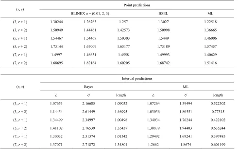
er record values _T*_{when (}_p_{= 0.4,}_θ_{= 1.24}915, θ = 3.19504, Table 1. Point and 95% interval predictors for the future upp

Ω = 0.5).

s 1 2

Point predictions (r, s)

BLINEX a = (0.01, 2, 3) BSEL ML

(3, r + 1) 1.30244 1.26763 1.257 1.3027 1.22518

(3, r + 2) 1.50949 1.44461 1.4257

(5, r + 1 54467 1.54467 1.5030

+ 1) 1.46631 1.4558 1.49993 1.40629

(7, r + 2) 1.68695 1.62164 1.6 1.68742 1.51416 3 1.50998 1.36665

3 1.5449 1.46006

) 1.

(5, r + 2) 1.73144 1.67009 1.65177 1.73189 1.57457

(7, r 1.4997

0205

Interval predictions

Bayes ML (r, s)

L U length L U length

(3, r + 1) 1.07653 2.16685 1.09032 1.07264 1.59494 0.522302

(3, r + 2) 1.14454 2.61449 1 1.0303 1.80551 515

1 1.3403 1.76244 102

(5, r + 2) 1.41102 2.76539 1. 7 1.30879 1.94403 0.635244

(7 ) 1.30032 2.31374 1.01 92 1.69241 0.397485

(7, r + 2) 1.37071 1.34801 1.2662 1. 0.601199

.46995 6 0.77

(5, r + 1) 1.34499 2.34997 .00498 4 0.422

3543

, r + 1 342 1.294

(9)

Table 2. Point and 95% inte redictors fo he future up values when (p = 0.391789, θ1 = 0.307317, θ2 =

3.33166, 5).

t predictio

rval p r t per record *

s

T

Ω = 0.

Poin ns (r, s)

(3, r + 1) 2.322 2.23435 2.21354 2.32287 2.21747

(3, 2) 2.68054 2.52154 2.48465 2.68226 2.4958

(5, 1) 2.81243 2.74901 2.73223 2.813 2.74014

2.66724 2.62719 2.61879 2.6678 2.62507

(7, r + 2) 2.8745 2.79894 2.7 2.87574 2.79966

r +

(5, r + 2) 3.13233 3.01438 2.98352 3.13346 3.00112

(7, r + 1)

8385

Bayes ML (r, s)

L U length L U length

(3, r + 1) 1.91839 4.03255 .11416 2 1.91487 2.94288 1.02801

(3, r + 2) 1.80949 5 3. 1.8297 3.35066 09

4 1 2.4633 3.42614 751

5 2 2.5306 3.82785 24

(7, r + 1) 2.44491 3.71097 1.26605 2.44436 3.08759 0.643231

(7, r + 2) 2.39459 4.67043 2.27 746 3.37074 0.97328

.02409 2146 7 1.52

(5, r + 1) 2.46589 .17173 .70584 9 0.962

(5, r + 2) 2.54923 .01563 .46641 1 1.297

584 2.39

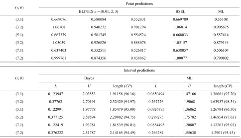
Table 3. Point and 95% interval predictors fo e future upp rd values Y b = 1, 2 when ( 0.4, θ1 = 1.2 2 =

3.1950 5).

int predictio

r th er reco *

b , p = 4915, θ

4, Ω = 0.

Po ns (r, b)

(3.1) 0.669076 0084 0.58 0.552831 0.669789 0.55108

(3.2) 1.06708 0272 0.901294 1.068

9 1745 0.554524 0.668 0.

(5.2) 1.05059 0.926826 0.888678 1.05157 0.879144

(7.2) 0.999761 0.874356 0.838862 1.00077 0.790802

0.94 14 0.905675

(5.1) 0.66737 0.58 033 557414

(7.1) 0.637403 0.552511 0.526817 0.638057 0.506104

Bayes ML

(r, b)

L U length (CP) L U length (CP)

(3.1) 0.123947 2.03553 1.91158 (96.16) 0.0850494 1.47166 1.38661 (97.70)

(3.2) 0. 2.70 2.32429 (94. 0.267226 068 1.

0. 1.97 1.85479 (95. 0.0926795 062 1.

0. 2.58 2.20882 (94. 0.289275 782 1.

(7.1) 0.122419 1.93781 1.81539 (96.01) 0.0854495 1.20807 1.12263 (95.03)

0.376222 2.51787 2.14165 284 1.55638 1.2901 (95.43)

37762 191 97) 1.9 63957 (98.54)

(5.1) 122991 778 90) 1.36 26794 (96.50)

(5.2) 377125 594 75) 1.75 46854 (97.63)

(10)

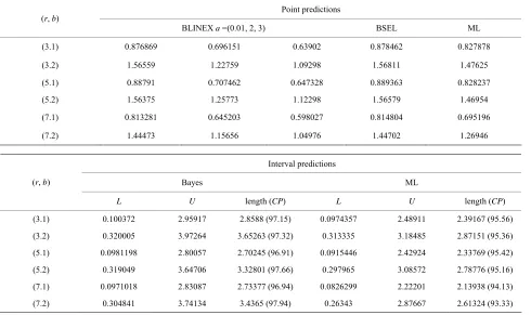
Table 4. Point and 95% interval predictors future upper record values * b

Y , b = 1, 2 when ( .391789, θ1 = 0.307317,

θ2 = 3.33166, Ω = 0.5).

predi

for the p = 0

Point ctions (r, b)

a =(0. BSEL

BLINEX 01, 2, 3) ML

(3.1) 0.876869 0.696151 0.63902 0.878462 0.827878

(3.2) 559 22759 09298 1.5681

) 0. 1 707462 647328 0.889363

) 375 25773 12298 1.5657

(7.2) 1.44473 1.15656 1.04976 1.44702 1.26946

1.56 1. 1. 1 1.47625

(5.1 8879 0. 0. 0.828237

(5.2 1.56 1. 1. 9 1.46954

(7.1) 0.813281 0.645203 0.598027 0.814804 0.695196

Bayes ML (r

L U length (CP) L U )

, b)

length (CP

(3.1) 0.100372 2.95917 2.8588 (97.15) 0.0974357 2.48911 2.39167 (95.56)

(3 0.3200 3.97264 65263 (97.32) 313335 5 36)

(5 0.0981 2.80057 5 (96.91 446 4 5.42)

(5 0.3190 3.64706 32801 (97.66) 297965 2 16)

(7.1) 0.0971018 2.83087 2.73377 (96.94) 0.0826299 2.22201 2.13938 (94.13)

(7.2) 0.304841 3.74134 3.4365 ( 343 2.87667 2.61324 (93.33)

.2) 05 3. 0. 3.1848 2.87151 (95.

.1) 198 2.7024 ) 0.0915 2.4292 2.33769 (9

.2) 49 3. 0. 3.0857 2.78776 (95.

97.94) 0.26

known and (72) and 73) wh ( en p and j are un-known.

6) T PP for the er is co

puted b on L usi p

know 4)

he B future obs

1) vatio

Point and 95% interval pr for fut r- ns are ob ned using a on sample an le

es b MTR ion. e

lized record v

is ev m all tab at, the length e nd BPI as th le size increase.

r fi ple size length I

PI in increasi

edictors e

-ure obse d two-samp tai

schem ased on a distribut Our results ar specia to upper alues.

2) It MLPI a

ident fro decrease

les th e samp

s of th

3) Fo xed sam r the s of the MLP and B crease by ng s o

vati ng (

on yb, m-

ased BSE 61) when is

when

function

n and (7 p and j ar unk

7) T PP for th ervat is co

puted b on BL on usi hen

is know 6)

e nown. ion y ,

he B e future obs b

ng (63) w m-

ased INX

whe

loss functi p

n and (7 n p and j ar n. 8) Ge 10, 000 sam each of size 6 from TR d tion, then calcu e cove rcentag

w m

n, e unknow nerate

istribu

ples late th

N = rage pe

a e

r b.

The pe e covera ves b e

number of observed values.

CES

ps, “A Concep

4) rcentag ge impro y use of a larg M

(CP) of Yb.

The computational (our) results ere co puted by using Mathematica 7.0. When p is know the prior parameters chosen as ₁2.3,₂2.7,₁0.5,₂1.3

which yield the generated values of ₁1.24915 and

2 3.19504

  . While, in the case of four parameters are unknown the prior parameters



b b c c d d₁, , , , ,₂ ₁ ₂ ₁ ₂



cho-

sen as



1.2, 2.3, 2, 2,0.3,3



which yield the generat va

REFEREN

[1] U. Kam t of Generalized Order Statistics,” Journal of Statistical Planning and Inference, Vol. 48, No. 1, 1995, pp. 1-23.

doi:10.1016/0378-3758(94)00147-N

[2] M. Ahsanullah, “Generalized Order Statistics from Two rm Distribution,” Communications in Sta- nd Methods, Vol. 25, No. 10, 1996, pp.

.1080/03610929608831840

ed

Parameter Unifo tistics—Theory a lues of p0.391789, ₁0.307317,₂3.33166.

In Tables 1-4 point and 95% interval predictors for the future upper record value are computed in case of the on

2311-2318. doi:10

[3] M. Ahsanullah, “Generalized Order Statistics from Expo- nential Distributiuon,” Journal of Statistical Planning and Inference, Vol. 85, No. 1-2, 2000, pp. 85-91.

doi:10.1016/S0378-3758(99)00068-3 [4] U. Kamps and U. Gather, “Cha e- and two sample predictions, respectively.

5.3. Conclusions