Dynamic Divisible Load Balancing Algorithm for
Balancing Workload in Cloud Computing
Neetu
Department of Computer Science & Engineering Rajasthan College of Engineering for Women
Bhankrota, Ajmer Road, Jaipur - 302026
Subhash Chandra
Assistant Professor, Department of Computer Science & Engineering
Rajasthan College of Engineering for Women Bhankrota, Ajmer Road, Jaipur - 302026
ABSTRACT
One of the developing zones in the field of data innovation is Cloud Computing. Cloud computing is a term which includes virtualization, systems services, programming and web services. Cloud computing helps to share data and provides many resource to users.It incorporates adaptation to internal failure, high accessibility, adaptability, decreased overhead for clients, reduced expense of proprietorship, on interest administrations and so forth. Load balancing is a central challenge in cloud computing because measure of information storing increments rapidly in open environment. Load balancing is a way toward redistributing the workload among Datacenters to improve both asset use and job reaction time. Load balancing aids to allocate the static / dynamic workload across numerous nodes to guarantee that no solo node is overloaded.Several existing algorithms deliver load balancing and improved resource utilization. There are several type of loads are possible in cloud computing like memory, CPU and network load. The work presented in this paper provides better algorithm for balancing loads in cloud environment. The methodology adopted for this dissertation has minimized the make span time of the system and got better throughput of the system. The tool used to prove this work is CloudSim with integrated development environment as Java Eclipse.
Keywords
Load Balancing, Datacenter, Broker, Host, Cloud Virtualization, CloudSim, Dynamic load balancing, Load balancing Algorithm.
1.
INTRODUCTION
In today scenario, Cloud computing is a buzzword in IT industry and many are interested to know what cloud computing is and how it works. Cloud computing is a technique to deliver information technology services on demand over a network rather than physically having the computing resources at the client location, in which resources are recovered from the Internet through online tools and applications. It permits us to manipulate, arrange and get to hardware and programming resources remotely. It offers online information storage, system and application. In other words, we can say cloud computing is a collection of servers which delivers services on demand. The cloud based services decrease the cost of hardware and software for the establishment of IT industry. Cloud computing is a strategy to upgrade the limit or include abilities powerfully without putting resources into new foundation, preparing newcomers, or buying new programming. Cloud computing includes the idea of cloud computing aside from that it gives on interest resources provisioning.
The demand of cloud based services raised some issue like load balancing related to the cloud computing environment.
The set number of resource and boundless number of demand makes some over-burdening situation in cloud. It is focused to give better usage of resources using virtualization process.
1.1
Load Balancing
Load balancing can be characterize as a strategy for dispersing workload on the different PCs or a PC bunch through network links to accomplish ideal resource use which boosts throughput and limits generally speaking reaction time. It limits the total waiting time of the resources just as dodges an excessive amount of over-burden on the resources. In this technique, traffic is divided among servers, so that data can be sent and received without maximum delay.
One of the significant problem in cloud computing is to partition the workload dynamically. Total processing time required by a machine to implement whole the assigned jobs to that machine is termed as workload for that machine [13]. Load balancing is a method to improve the performance of a system by shifting the workload among all the processors [14]. The profits of distributing the workload includes higher resource utilization ratio which further leads to improving the whole performance thereby attaining maximum client fulfillment. Subsequently load balancing is one of the significant factors to boost the working performance of the cloud service provider.
1.1.1
Classification of Load Balancing Algorithm
Based on process orientation, load balancing algorithms are classified as: Sender Initiated
Receiver Initiated
Symmetric
Sender Initiated: In this category sender starts the process; the client sends request for until a recipient is allocated to him to get his remaining task at hand. For example the sender starts the process.
Receiver Initiated: The receiver starts the procedure; the recipient sends a solicitation to recognize a sender who is prepared to share the workload for example the receiver starts the procedure.
Symmetric: It is a mixture of both sender and receiver started kind of load balancing algorithm.
The process based on the current state of the system, load balancing algorithms can be classified as:
a) Static Load Balancing
Static Load Balancing
In the static load balancing algorithm the choice of moving the load does not depend upon the current scenario of the system. These algorithms needn't bother with the data in regards to current environment of the system. This kind of algorithms has serious drawbacks in the event of sudden disappointment of system resource, assignments and furthermore undertaking can't be shifted during its execution for load balancing. Static load balancing algorithms are not pre-emptive and in this way each machine has no less than one task allocated for itself. The four distinct sorts of Static load balancing process are Round Robin algorithm, Central Manager Algorithm, Threshold algorithm and randomized algorithm.
Dynamic Load Balancing
Dynamic Load Balancing algorithms [9] are choice concerning load balancing dependent on the present environment of the system. There is no requirement of any prior information about the system. This will overcome the disadvantages of static methodology. This means it takes into consideration process pre-emption which isn't supported in Static load balancing approach. The dynamic algorithms are complex; however they can give better execution and adaptation to non-critical failure. A critical favorable position of this methodology is that its choice for balancing the load depends on the present environment of the system which helps in improving the general execution of the system by relocating the load powerfully.
1.2
Virtualization in Cloud
Virtualization means which are not exist in real, but it provides everything like real. Virtualization is the software implementation of a machine which executes different programs like a real machine. Through the virtualization user can use the different applications or services of the cloud, so this is the main part of the cloud environment.
There are two different types of virtualization is used in cloud environment.
a) Full virtualization
b) Para virtualization
Full Virtualization: Full virtualization means a complete machine is installed on another machine which provides all those functions which exist on the original machine.
Para virtualization: Para virtualization means the hardware allows numerous operating systems to run on single machine. It allows efficient use of system resources such as memory and processor.2.
RELATED WORK
Multiple static and dynamic algorithms have been proposed in previous decade. Static algorithms allocate workload among processors before execution of algorithm and hence require prior knowledge of the system state. These algorithms give better results only when there is minimum variation in upcoming workload. J.Li et. al., [1] and B.Sahoo et. al., [2] both use the greedy approach to reduce the makespan time and execution time without using any load balancing approach (task migration or virtual machine migration), both approach do not work well in real environment. Greedy based algorithm [2] gives better results than [1] because this algorithm follows the dynamic approach. P.Samal and P.Mishra proposed round robin procedure considering the parameter reaction time and asset usage to tackle the issue of load balancing in cloud
environment [3] yet algorithm don't limit the reaction time and makespan time. All discussed algorithm are not appropriate for real time environment like cloud computing where load on each node vary very habitually i.e., we cannot forecast the coming load therefore we need a dynamic algorithm. There is no requirement of advanced information about the resource and task in dynamic algorithm because this type of algorithm constantly observes the resource.
A.Lakra and D.Yadav [4] proposed an algorithm to decrease turnaround time, cost and enhance throughput parameter. Abdulhamid, AbdLatiff et al. [5] have assessed chosen scheduling algorithms dependent on the parameters, for example, load balancing, energy consumption, and make span and so forth. They concluded that none of the checked on scheduling algorithms satisfy the whole scheduling parameter necessities. Be that as it may, their audit assessed assignment scheduling algorithms and furthermore there is a gap for examining the open issue and difficulties in their survey. Jing Tai Piaoet. al. [6] inside the implement, they depicted approach places the VMs on physical machines with observation of the network things between the data storage and thus the physical machines. Throughout the implement, their strategy has in addition monitored the concept throughout that instable network situation changed the data access behaviors and deteriorated the appliance performance, and prohibited this idea by migrating the VM to totally different physical machines. All through the actualize, their system has what's more checked the idea all through that instable system circumstance changed the information get to practices and weakened the apparatus execution, and restricted this thought by moving the VM to very surprising physical machines. The simulation result on CloudSim 2.0 shown the mentioned strategy may update the task completion time.
D. Chitra Devi et. al. [7] worked on Load Balancing in Cloud Computing surroundings using Improved Weighted Round Robin Algorithm for No preemptive Dependent Tasks. According to [8] Cloud computing usages the concepts of scheduling and load balancing to transfer jobs to underused VMs for efficiently sharing their sources. The taking part heterogeneous resources are overseen by designating the undertakings to fitting resources by static or dynamic scheduling to make the cloud computing progressively effective and hence it improves the client fulfillment. Goal of this work was to present and assess the proposed scheduling and load balancing calculation by considering about the capacities of each virtual machine(VM), the task length of each requested job, and the inter dependency of multiple tasks. Performances of the planned algorithm were studied by comparing with the existing methods. We have proposed and develop a dynamic load balancing algorithm that minimizes the make span time of the system and get better throughput of the system.
3.
PROPOSED WORK
We have proposed a dynamic divisible load balancing algorithm in case of clouds is an optimal division of loads among datacenters, whose objective is to reduce, make span time and increase average resource utilization ratio in cloud environment. We created number of datacenter host and broker by using CloudSim tool.
3.1
Algorithm and Technique
Host Load = Host Bandwidth + Host RAM + Host CPU time
VM Load = VM Bandwidth + VM RAM + VM CPU time
Cloudlet weight = cloudlet length + input file size + output file size.
Now, we assign priority to the cloudlets and arrange the cloudlets accordingly. If any cloudlets have same priority then cloudlet with least weight will come first. Also arrange the Host and VMs according to their loads in ascending order.
For allocating VMs to host, in arranged VM and Host check if the VM load is less than the host load and if yes, then allocate the VM to the host else check another host. After allocation subtract the allotted VM load from the allotted host load. For allocating cloudlets to VM, we have defined a least bound, which is given as:
Least Bound = ceil (number of cloudlet / number of VM)
Also, we keep tracking the number of cloudlets connected to each VM and make sure it will not exceed the least bound value.
In arranged cloudlets and VM check if cloudlet weight is less than the VM load, also check if number of connected cloudlets to that VM is less than or equal to the least bound then allocate cloudlet to the VM, else check for another VM. After allocation update the number of connection of the allotted VM and subtract the allotted cloudlet weight from the allotted VM load.
We have calculated the estimated VM duration by dividing the VM load by the available computer resources.
Estimated VM duration = VM load / (Host CPU time + Host RAM + HOST Bandwidth)
Similarly, we have calculated the estimated cloudlet duration by dividing cloudlet weight by the available VM resources.
Estimated cloudlet duration = cloudlet weight / (VM CPU time + VM RAM + VM Bandwidth).
We have also calculated the throughput of the system as,
Throughput = Number of cloudlet / total time taken.
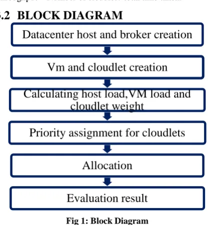
[image:3.595.59.268.510.736.2]3.2
BLOCK DIAGRAM
Fig 1: Block Diagram
In figure 3.2.1, data flow diagram shows the process of proposed algorithm.
3.3
Environment execution
Module 1: Datacenter host and Broker creation
Firstly, number of Datacenter host and Broker will be created which is done using the CLOUDSIM tool.
Step 1: Start.
Step 2: Declare variable nofdatacenter and nofbroker creation.
Step 3: Read nofdatacenter and nofbroker.
Step 4: For i = 1 to nofdatacenter
Call CreateDatacenter(i)
Step 5: Create Datacenter
Declare variable nofmachine.
Read random value of nofmachine from 2 to 5.
For j = 1 to nofmachine
Call Host from CLOUDSIM library.
Declare variable ram, bw, storage and host_id.
Initialize host_id as 0.
Read random values of ram, bw and storage.
host_id = host_id +1
Step 6: For k = 1 to nofbroker
Call CreateBroker
Step 7: CreateBroker
Declare variable dcb.
dcb=call Datacenter Broker class from CLOUDSIM library.
Step 8: Stop.
Module 2: VM and cloudlet creation
VM and cloudlet will be created using the CLOUDSIM tool. Step 1: Start.
Step 2: Declare variable nofvm and nofcloudlet. Step 3: For i = 1 to nofvm
Call VM class from CLOUDSIM library. Step 4: For j =1 to nofcloudlet
Call Cloudlet class from CLOUDSIM library. Step 5: Stop.
Module 3: Host Load, VM Load and cloudlet weight algorithm.
Now, Host Load, VM Load and cloudlet weight will be calculated by cloud provider for further allocation of load to the server.
Step 1: Start.
Step 2: Declare variables h_cpu, h_mips, h_ram, vm_cpu, vm_mips, vm_ram, c_length, c_input_file, c_output_file, host_load, vm_load and cloudlet_weight.
Step 3: Read values h_cpu, h_mips, h_ram, vm_cpu, vm_mips, vm_ram, c_length, c_input_file and c_output_file. Step 4: Add h_cpu, h_mips and h_ram and assign the result to host_load.
Step 5: Add vm_cpu, vm_mips and vm_ram and assign the result to vm_load.
Step 6: Add c_length, c_input_file and c_output_file and assign the result to cloudlet_weight.
Step 7: Stop.
Module 4: Arranging Host Load and VM Load. Host Load and VM Load is arranged in ascending order.
Datacenter host and broker creation
Vm and cloudlet creation
Calculating host load,VM load and
cloudlet weight
Priority assignment for cloudlets
Allocation
Step 1: Start.
Step 2: Declare array host_load [ ] and vm_load [ ].
Step 3: Declare variable temp, nofhost and nofvm.
Step 4: Read values nofhost and nofvm.
Step 5: For i = 1 to nofhost
Read host_load [ ]
Step 6: For j = 1 to nofvm
Read vm_load [ ]
Step 7: For k = 1 to nofhost
If host_load [k] >host_load [k+1]
temp = host_load [k]
host_load [k] = host_load [k+1]
host_load [k+1] = temp
Step 8: For l = 1 to nofvm
If vm_load [l] >vm_load [l+1]
temp = vm_load [l]
vm_load [l] = vm_load [l+1]
vm_load [l+1] = temp
Step 9: Stop.
Module 5: Allocating VM to Host and finding estimated duration of VM
Now, we apply the algorithm for allocating VM to Host. After which we evaluate estimated duration of VM.
Step 1: Start.
Step 2: Declare array vm_duration [ ] and final_vm [ ].
Step 3: Declare variable temp.
Step 4: For i = 1 to nofvm
For j = 1 to nofhost
If vm_load [i] <host_load [j]
Allocate VM to the host.
final_vm [k] = i
k = k + 1 vm_duration [i] = vm_load[i] / host_load[j]
temp = host_load [j]
host_load [j] = temp – vm_load [i]
Step 5: Stop.
Module 6: Arranging cloudlets
Now, cloudlet will be arranged according to the assigned priority and if any cloudlet have same priority then cloudlet with minimum weight will come first.
Step 1: Start.
Step 2: Declare an array priority.
Step 3: Read values of priority [ ].
Step 4: Declare variable nofcloudlet, temp1 and temp2.
Step 5: Read value of nofcloudlet.
Step 6: For i = 1 to nofcloudlet
Read cloudlet_weight [ ].
Step 4: For j = 1 to nofcloudlet
If priority [j] > priority [j+1]
temp1 = priority [j]
priority [j] = priority [j+1]
priority [j+1] = temp1
temp2 = cloudlet_weight [j]
cloudlet_weight [j] = cloudlet_weight [j+1]
cloudlet_weight [j+1] = temp2
else if priority [j] = priority [j+1]
if cloudlet_weight [j] >cloudlet_weight [j+1]
temp2 = cloudlet_weight
[j]cloudlet_weight[j]=cloudlet_weight [j+1]
cloudlet_weight [j+1] = temp2
Module 7: Allocating cloudlet to VM, finding estimated duration of cloudlet and finding total estimated duration Now, algorithm is applied to allocate cloudlet to capable VM server. After which estimated cloudlet duration is evaluated and total estimated duration will be obtained by the summation of estimated VM duration and estimated cloudlet duration.
Step 1: Start.
Step 2: Declare array cloudlet_duration [ ], total_duration and active [ ].
Step 3: Declare variable temp1, temp2, vm_dur and least_bound.
Step 4: For m = 1 to nofvm
active [m] = 0
Step 5: least_bound = ceil (nofcloudlet / nofvm)
Step 4: For i = 1 to nofcloudlet
For j = 1 to nofvm
If cloudlet_weight [i] <vm_load [j] and active [j] <= least_bound
Allocate cloudlet to the VM.
cloudlet_duration [i] = cloudlet_weight[i] / vm_load[j]
temp1 = vm_load [j]
For k = 1 to final_vm
If final_vm = j
vm_dur = vm_duration [k]
total_duration [i] = vm_dur + cloudlet_duration
vm_load [j] = temp – cloudlet_weight [i]
temp2 = active [j]
active [j] = temp2 + 1
Step 5: Stop.
Throughput is the rate at which number of cloudlet get finished per unit time.
Step 1: Start.
Step 2: Declare variable throughput, finish_time and temp.
Step 3: For i = 1 to nofcloudlet
temp = total_duration [i]
finish_time = finish_time + temp
Step 4: throughput = nofcloudlet / finish_time
Step 5: Stop.
4.
RESULTS ANALYSIS
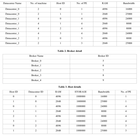
After applying our algorithm let’s find the result for the following scenario:
Number of Datacenter = 3.
Number of Broker = 5.
Number of VM = 7.
Number of cloudlet = 10.
[image:5.595.57.540.224.694.2]4.1
Evaluation
Table 1. Datacenter detail
Datacenter Name No. of machine Host ID No. of PE RAM Bandwidth
Datacenter_0 2 0 1 4096 16000
Datacenter_0 2 1 1 2048 25000
Datacenter_1 4 0 4 4096 24000
Datacenter_1 4 1 4 2048 8000
Datacenter_1 4 2 4 4096 8000
Datacenter_1 4 3 4 2048 24000
Datacenter_2 2 0 3 4096 8000
Datacenter_2 2 1 3 2048 25000
Table 2. Broker detail
Broker Name Broker ID
Broker_0 5
Broker_1 6
Broker_2 7
Broker_3 8
Broker_4 9
Table 3. Host details
Host ID Datacenter ID RAM STORAGE Bandwidth No. of PE
0 0 4096 1000000 16000 1
1 0 2048 1000000 25000 1
0 1 4096 1000000 24000 4
1 1 2048 1000000 8000 4
2 1 4096 1000000 8000 4
3 1 2048 1000000 24000 4
0 2 4096 1000000 8000 3
Table 4. VM details
VM ID Bandwidth RAM MIPS No. of PE
0 2000 1024 76 2
1 1000 3072 278 2
2 1000 2048 553 2
3 5000 3072 705 2
4 2000 512 499 2
5 1000 3072 785 2
6 5000 2048 381 2
Table 5. Host Load
Host ID Datacenter ID LOAD
0 0 20595
1 0 48142
0 1 32732
1 1 47416
2 1 64148
3 1 94832
0 2 16587
1 2 48126
Table 6. VM Load
VM ID LOAD
0 3100
1 7450
2 11051
3 19828
4 22839
5 27696
6 35125
Table 7. Allotted host to VM
Datacenter ID Host ID VM ID
2 0 0
2 0 1
0 0 2
1 0 3
1 1 4
2 1 5
[image:6.595.324.528.248.468.2]0 1 6
Table 8. Cloudlet Priority assignment
Cloudlet ID Weight Priority
8 282 0
1 1007 0
7 555 2
3 666 2
9 709 5
0 760 5
2 777 5
5 336 7
6 566 7
[image:6.595.322.536.489.727.2]Table 9. Allotted cloudlet to VM
VM ID Cloudlet ID
0 8
0 1
0 7
1 3
1 9
1 0
2 2
2 5
2 4
[image:7.595.318.542.302.435.2]3 6
Table 10. Evaluated result
Cloudlet ID Flow Time Start Time Finish Time
8 0.27786 0 0.27786
1 0.54424 0.27786 0.82210
7 0.49335 0.82210 1.31545
3 0.64178 1.31545 1.95723
9 0.65689 1.95723 2.61412
0 0.67748 2.61412 2.29160
2 0.60690 2.29160 3.89850
5 0.56929 3.89850 4.46779
6 0.59354 4.46779 5.06133
4 0.67870 5.06133 5.74003
4.2
Calculating make span time
Make span time = Summation of flow time of all cloudlet
Make span time = 5.74003
4.3
Calculating throughput
Throughput = number of cloudlet / make span time
Throughput = 10 / 5.74003
Throughput = 1.74215
4.4
Analyzing throughput
Series 1:
Number of Datacenter = 13.
Number of Broker = 15.
Number of VM = 20.
Series 2:
Number of Datacenter = 15.
Number of Broker = 17.
Number of VM = 15.
Series 3:
Number of Datacenter = 14.
Number of Broker = 16.
Number of VM = 17.
Figure 4.4.1 shows the throughput graph of the above cases with four different numbers of cloudlets 30, 60, 90 and 120. X-axis shows the number of cloudlets whereas Y-axis shows the throughput of the system. Client provides the number of Datacenter, Broker, VM and cloudlet. Each Datacenter creates number of hosts depending on the algorithm and cloud provider calculate the loads and allocate to the capable server according to the implemented algorithm. And throughput is evaluated accordingly.
Fig 2: Performance evaluations according to throughput
5.
CONCLUSION AND FUTURE SCOPE
This paper provides knowledge to get familiar with the available CloudSim packages which help in implementing any load balancing algorithm. Using this algorithm, throughput can be maintained. Overall, the end goal of forwarding the incoming cloudlets to the capable server has been achieved. And with this proposed work provides a lot about cloud computing and load balancing, especially for those who never had much insight in such vast topic.
This proposed work can be further extended to be applied on load migration environment. This proposed work can also be extended to provide strength check of the system i.e., if any of the server is failed then the algorithm will stop sending cloudlet to that server. Also, this algorithm can be applied on pre-emptive system with little changes.
6.
REFERENCES
[1] Ji.Li, Longhua Feng, Shenglong Fang, “An Greedy-Based Job Scheduling Algorithm in Cloud Computing”, Journal of Software, Vol. 9, No. 4, April 2014.
[2] Bibhudatta Sahoo, Dilip Kumar and Sanjay Kumar Jena “Analysing the Impact of Heterogeneity with Greedy Resource Allocation Algorithms for Dynamic Load Balancing in Heterogeneous Distributed Computing System,” IJCA Impact of Hetroginity, Jan. 2013. [3] P. Samal and P. Mishra “Analysis of variants in Round
[image:7.595.56.279.371.560.2]Computing,” International Journal of Computer Science and Information Technologies, 2013.
[4] A. Lakra, and D. Yadav, "Multi-Objective Tasks Scheduling Algorithm for Cloud Computing Throughput Optimization", Procedia Computer Science, 2015.
[5] Sim Abdulhamid, A Latiff, M Shafie, "Scheduling techniques in on-demand cloud as a service cloud: A review", Journal of Theoretical and Applied Information Technology 63: 10--19.
[6] Jing Tai Piao and Jun Yan “A Network-aware Virtual Machine Placement and Migration Approach in Cloud Computing”, IEEE, 2010, Pp 87-92.
[7] D. Chitra Devi and V. Rhymend Uthariara, “Load Balancing in Cloud Computing Environment Using Improved Weighted Round Robin Algorithm for Non-preemptive Dependent Tasks”, Hindawi Publishing Corporation e Scientific World Journal Volume 2016, PP 1-14.
[8] Sandeep Joshi and Pradeep Kumar Tiwari. "Load management using virtual machine migration." International Journal of Advanced Computer Communications and Control Vol. 03, No. 01, January 2015.
[9] Ray, Soumya, and Ajanta De Sarkar, “Execution analysis of load balancing algorithms in cloud computing environment”, International Journal on Cloud Computing: Services and Architecture (IJCCSA) 2.5 (2012): 1-13.
[10] Peter Mell and Timothy Grance, “The NIST Definition of Cloud Computing”, NIST Special Publication 800-145.
[11] Dr. Neenu Juneja, Krishan Tuli and Sarabjeet Kaur, “Load Balancing Techniques in Cloud Computing”, International Journal for Scientific Research & Development Vol. 4, Issue 12, 2017 ISSN (online):2321-0613.
[12]Rajwinder Kaur and Pawan Luthra, “Load Balancing in Cloud Computing”, Proc. of Int. Conf. on Recent Trends in Information, Telecommunication and Computing, ITC.
[13] Nitin Kumar Mishra and Nishchol Mishra, “Load Balancing Techniques: Need, Objectives and Major Challenges in Cloud Computing- A Systematic Review”, International Journal of Computer Applications (0975 – 8887) Volume 131 – No.18, December 2015.
[14] Kaushal M. Madhu and S. M. Shah, “Study on Dynamic Load Balancing in Distributed System”, International Journal of Engineering Research & Technology (IJERT) Vol. 1 Issue 9, November- 2012 ISSN: 2278-0181
[15]Sukhvir Kaur and Supriya Kinger, “Review on Load Balancing Techniques in Cloud Computing environment”, International Journal of Science and Research (IJSR) ISSN (Online): 2319-7064 Impact Factor (2012): 3.358.