Sensitivity Analysis of Parameters in Water Quality
Models and Water Environment Management
Dongjun Liu, Zhihong Zou*
School of Economics and Management, Beihang University, Beijing, China. Email: *[email protected]
Received June 15th, 2012; revised July 10th, 2012; accepted August 9th, 2012
ABSTRACT
The impacts of changes of various parameters and stochastic factors on water quality models were studied. The impact of deviation of the degradation coefficient on the model results was investigated. The degradation coefficient was de-composed into the exact part and the deviation part, and the relationship between the errors of the water quality model results and the deviation of the degradation coefficient was derived. The impact of changes in the initial concentration on the model results was discussed. A linear relationship between the initial concentration changes and errors in the model results was obtained, and relevant recommendations to the water quality management were made based on the results. The impacts of stochastic factors in the water environment on the water quality model were analyzed. A variety of random factors which may affect the water quality conditions were attributed to one stochastic factor and it was fur-ther assumed to be the white noise. The solutions to the water quality model including the stochastic process were ob-tained by solving the stochastic differential equation. Simulation results showed that the decay trend of the concentra-tion of the solute would not be changed, and that the results would fluctuate around the expectaconcentra-tion centered at each corresponding displacement x.
Keywords: Water Quality Model; Reclaimed Water; Sensitivity Analysis; Degradation Coefficient; Stochastic Factors
1. Introduction
With the development of economies and the improve-ment of living standards, our environimprove-ment, especially natural water, is constantly being polluted. Natural water plays an important role in a watershed in carrying off municipal and industrial wastewater and run-off from farm land. In recent years, water pollution and water shortages are two of the most serious and widespread environmental problems [1]. The application of re-claimed water is of great importance to ease the water shortage and reduce further pollution by sewage. The use of reclaimed water as an unconventional supply for rivers with water shortages has become a common and interna-tional trend [2]. The recycled water comes from urban sewage which has been extensively treated in sewage treatment plants. Although it may meet certain water quality standards, it is still urban sewage and carries some risk when used to recharge rivers. Therefore, study of the analysis and management of the water quality of rivers recharged with reclaimed water has high theoreti-cal and practitheoreti-cal significance [3].
The theoretical study of water quality management has
the goal of developing mathematical models based on real water quality. Conclusions and information on water quality changes have been obtained by discussing and analyzing these models [4]. The history of study on water quality models can be divided into three stages according to the complexity and perfection of the models.
The first stage was from the 1920s to the early 1970s, when the models were simple oxygen balance models. This stage was the early stage of development of surface water quality models [5]. The models during this phase mainly focused on the study of the oxygen balance, but also involved some non-ozone-depleting substances. The starting point of this research phase was the BOD (Bio-chemical Oxygen Demand)-DO (Dissolved Oxygen) coupled equation which was proposed by Streeter and Phelps in 1925, designated the S-P equation [6]. In the next few decades, there were scientists who proposed an amendment to the S-P equation. Theriault (1927) [7] and Fair (1939) [8] summarized the methods for estimating the model’s parameters. To account for the removal through sedimentation of the settleable BOD, Streeter (1935) [9] realized its consideration; Thomas (1937, 1948) [10,11] considered (though less elegantly) this effect through use of a “lag-time”. In 1961, O’Conner
insisted that BOD should be divided into two parts, namely CBOD at the carbonation stage and NBOD at the nitrification stage, and that the reduction of DO should also be the sum of these two parts. Thus the model was modified based on the S-P equation, after considering the impact of the nitrification process on the changes of DO [12]. Clark and Viessman (1965) [13] pointed out that second-order rather than first-order reactions frequently describe the stabilization of waste-waters. Braun and Berthouex (1970) [14] proposed a Michaelis-Menton expression to describe the BOD decay reaction and its impact on the DO concentration in a river. The S-P equa-tion and its modified model are still widely used.
The second stage was the mid-1970s to the 1990s, when comprehensive water quality models rapidly de-veloped [15]. With in-depth study on the environmental behavior of pollutants in water, the traditional oxygen balance model was found lacking and could not meet the actual needs. Other pollutants began to be considered in water quality models. The environmental behavior and ecological benefits of different forms of pollutants, as well as the distribution of pollutants in the air, water, soil and vegetation in a variety of environmental media, be-came research subjects. Therefore, river water quality needed to be described comprehensively, and it was nec-essary to study the link between aquatic ecosystems and water quality components; then comprehensive water quality models could be built [16]. Due to the develop-ment of computer science, a huge amount of computing had become possible at this stage. Models were develop-ing from one-dimensional to multi-dimensional, and they were closer to real systems.
The United States started the research on the compre-hensive water quality models in the early 1970s, and the QUAL model system was first proposed [17]. The QUAL-I model was developed by the Texas Water De-velopment Board with Frank D. Masch and Associates during 1970 to 1971 [18]. In June 1972, the United States Environmental Protection Agency awarded Water Re-sources Engineers, Inc. (now Camp Dresser & McKee) a contract to modify QUAL-I for application to the Chat-tahoochee-Flint River, the Upper Mississippi River, the Iowa-Cedar River, and the Santee River. The modified version of QUAL-I was known as QUAL-II [19]. The QUAL model system has been continually developed since then. In 1985, EPA’s Center for Water Quality Modeling sponsored a National Council of the Paper Industry for Air and Stream Improvement (NCASI) re-view of other versions of QUAL-II and incorporated cer-tain features of these versions into a program called QUAL2E [20]. QUAL2E is currently the best available stream model that has been adapted for use on a personal computer. The model is numerically accurate and in-cludes an updated kinetic structure for most conventional
pollutants. The QUAL2E model was widely used. In 2000, the model underwent further refinement and up-grade, and the QUAL2K version was introduced. This version could be loaded into Excel in the form of macros, and the model interface was also very user-friendly.
The third stage was the mid-1990s to the present, when surface water quality models were continuously deepened, improved and widely used. The water quality models had the following characteristics in this stage. Firstly, with increasing emphasis on non-point source pollution problems, the combination of the surface water quality model and non-point source pollution model be-gan to be considered. Secondly, the reliability and evalu-ation capacity of the models were strengthened, and more importance was attached to the models’ uncertainty. Fur-thermore, many modern mathematical methods were introduced into the research on water quality models, such as stochastic mathematics [21], fuzzy mathematics [22], artificial neural networks [23], genetic algorithms [24], expert systems [25], etc. Lastly, with the develop-ment of computer technology, 3S technology, that is, GIS [26] (Geographic Information System), RS [27] (Remote Sensing), and GPS [28] (Global Positioning System)) was introduced into the study on water quality models, which greatly promoted the development of model stud-ies.
In the current study, sensitivity analysis of the pa-rameters in water quality models was carried out. The influence of various parameters on the equation results were analyzed and discussed. The impact of changes in the parameters and random factors on the errors of the model results were investigated. The relationship be-tween these factors was verified by simulation results, and rational suggestions for water quality management were proposed.
2. Sensitivity Analysis of Water Quality
Model
2.1. Water Quality Model
A one-dimensional river flow dispersion equation for a pollutant was set as [29]:
2 2
s
C C C
u k k
t x x C
. (1)
where ks is the dispersion coefficient, k is the pollutant
degradation coefficient, C is the BOD concentration in water, x is the distance between the monitoring point and the source of pollution, and u is the flow rate.
River water quality at steady-state was considered. Uniform river section steady-state sewage conditions were the velocity and flow of cross sections that did not change with the time, that is, where C 0
t
tion (1) was transformed into Equation (2): 2 2 d d 0 d d s C C
k u kC
x
x . (2) Sensitivity analysis of the parameters in Equation (2) is discussed below.
2.2. Degradation Coefficient
When the dispersion effect is not considered, that is, ks =
0, Equation (2) transforms to Equation (3):
d d
C
u kC
x . (3) The initial condition is:
0 0
x
C C .
The degradation process of remaining BOD is:
0
k x u
C C e . (4) We decomposed k in Equation (4) into two parts:
1
k k k. (5) where k is the degradation coefficient, in d−1; k
1 is the exact part of k, in d−1; Δk is the deviation of k, in d−1, and Δk could be caused by measurement errors and uncertain factors.
We substituted Equation (5) into Equation (4), then
1 0 k k x x u u s
C C e e
. (6)
We expanded the power series of
k x u e : 2 1 2! kx u kx k u e x u .
We substituted the first two terms on the right side of the equation into Equation (6), then
1 1 0 0 k k x x u s k
C C e C x e
u
u . (7)
From Equation (7), the errors in the model results caused by Δk would be:
1 1 0 k x u k
E C x e
u
. (8)
[image:3.595.310.537.101.217.2]The impact of changes in the degradation coefficient on solute concentrations in water was investigated through the analysis of influence of Δk on E1, which was the sensitivity analysis of the degradation coefficient. After theoretical analysis, we used the data in a simula-tion to verify the model. The basic parameters of some rivers are shown in Table 1, from reference [30].
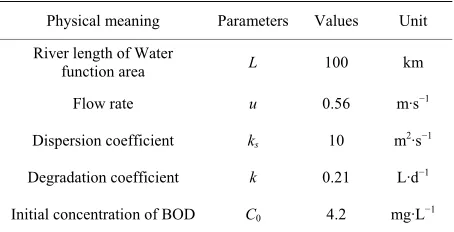
Table 1. Basic parameters of the river.
Physical meaning Parameters Values Unit
River length of Water
function area L 100 km
Flow rate u 0.56 m·s−1
Dispersion coefficient ks 10 m2·s−1
Degradation coefficient k 0.21 L·d−1
Initial concentration of BOD C0 4.2 mg·L−1
We substituted the water parameters in Table 1 into
Equation (7), and obtained the variation of the concentra-tion error E1 with the displacement x. We set Δk = 0.01 L·d−1, Δk = 0.005 L·d−1, Δk = 0.001 L·d−1 and Δk = −0.005 L·d−1 respectively, and plotted the variation of the error E1 with the displacement of x when Δk was set at different values, as shown in Figure 1.
From Figure 1 we can see that the concentration error
E1 decreased with increasing deviation of the degradation coefficient Δk. Considering absolute values, when k increased, E1 also increased. The signs of Δk and E1 were opposite. When Δk > 0, E1 < 0, and the value of Cs
would decrease from Equation (7); when Δk < 0, E1 > 0, and the value of Cs would increase from Equation (7).
We investigated the specific values of Δk and E1 at x = 4.0 km. According to Equation (8), when the degradation coefficient had increased 0.001 L·d−1, that is, Δk = 0.001 L·d−1, E
1 would decrease 0.0029 mg·L−1. This was equivalent to a situation where a 1% change in the deg-radation coefficient would cause about 0.15% error in the solute concentration. In addition, E1 was differentiated with respect to x and we calculated the derivative values. In the river length within functional areas, that was, x ≦
100 km, the derivative values were all less than 0. Thus we obtained the conclusion that E1 showed a monotoni-cally decreasing trend. When x increased, E1 would de-crease, and then Cs also decreased. Therefore, the im-pacts of Δk on E1 decreased gradually with increasing x.
2.3. Initial Concentration
In this section the impact of changes in the initial con-centration on the model results are discussed.
We solve Equation (2), then
21 4 1 1 2 0 s s k k ux k 0 x u
C x C e C e
. (9)
where 1 2 4 1 1 2 s s k k u k u .
Figure 1. Sensitivity analysis of degradation coefficient.
0 01 C C C0
1
. (10) We substituted Equation (10) into Equation (9), then
1 10 x 01 x 0 x C x C e C e C e .
Therefore, the error caused by the deviation of the ini-tial concentration ΔC0 was
1
2 0
x
E C e . (11) The impact of changes in the initial concentration on model results was investigated through the analysis of influence of ΔC0 on E2, which was the sensitivity analy-sis of the initial concentration. After theoretical analyanaly-sis, we again used the data for simulation to validate the model. Simulation parameters were the same as the ones used in Section 2.2.
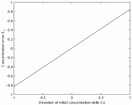
We substituted the parameters into Equation (11), and obtained the numerical relationship between E2 and ΔC0:
2 0.8406 0
E C .
We plotted the functional relationship between the er-ror E2 and the deviation ΔC0, as shown in Figure 2.
It was clear that there was a positive linear correlation between E2 and ΔC0. When ΔC0 increased, E2 also in-creased at the corresponding displacement x. This was because ΔC0 is the coefficient of E2 in Equation (11). Similarly, in Equation (8), C0 is the coefficient of C(x). There was also a positive linear correlation between C(x) and C0. When C0 increased, C(x) also increased at the corresponding displacement x.
On the other hand, according to the Water Quality Standards [31], a BOD concentration of 4.2 mg/L corre-sponds to Class III. For natural water, it is difficult to meet water quality requirements for this initial concen-tration. The concentration is officially required to decay back to 3 mg/L, which corresponds to Class I, by the self-purification of the river itself. The pollutant process
satisfied Equation (8), so that at least a 75 km distance would be needed if the water pollution began to decay from the initial concentration of 4.2 mg/L. The decay processes in the river are shown in Figure 3.
From Figure 3 we can see, if “3 mg/L”, which was the
[image:4.595.313.533.528.701.2]limiting value for Class I in Water Quality Standards, was actually required at a distance of 40 km from a pol-lution source, the water quality situation at present would not meet the requirements, and the concentration could not decay from the initial concentration of 4.2 mg/L to 3 mg/L at the 40 km. That means the water quality would need to be managed effectively. Reduction of the initial concentration at the pollution source is the most common and effective way to manage water quality. We imple-mented a reduction of the concentration at the pollution source, such that the initial concentration would be re-duced to 3.5 mg/L within 40 km. Thus “4.2 mg/L” was reduced by ΔC0 = 0.7 mg/L, and now the water quality
Figure 2. Concentration error and deviation of initial con-centration.
0 2 4 6 8 10
x 104 2
2.5 3 3.5 4 4.5
x/m
C
o
n
c
en
tr
at
io
n
/(
m
g/
L
)
began to change from an initial concentration of 3.5 mg/L. The concentration at the distance of 40 km could decay to the requirement of 3 mg/L though the river self-purification process, and its decay processes in the river are also shown in Figure 3. We calculated the
ini-tial concentration which could meet the requirement that concentration should decay to 3 mg/L at the 40 km dis-tance from the pollution source according to Equation (9). The result was C0 = 3.5687 mg/L.
2.4. Stochastic Factors
In this section the impact of stochastic factors in the wa-ter environment on the wawa-ter quality model are discussed. The stochastic factors in the water environment included: External or anthropogenic factors on the water environ-ment, uncertain measurement of parameters in the water quality model, the interaction and chemical reaction of the solutes, precipitation and drought and other climatic factors, etc. [32]. As we knew, when the dispersion effect was not considered, Equation (2) was transformed into Equation (3). We took stochastic factors into account in the water quality model. The integrity of the stochastic factors was seen as one factor, and we mainly considered the impact of this factor on the model [33]. Thus a sto-chastic factor “S” was added into the equation. Then Equation (3) was transformed:
d d
C
u kC S
x .
The stochastic factor “S” was assumed to be white noise with variance of σ2 [34], and “S” was represented by . Then the water quality model was transferred into a first-order constant coefficient linear stochastic differential Equation (12):
W x
uC x kC x W xd
. (12)
White noise could not be used as a stochastic process with a sample function in the usual sense, so Equation (12) was not determinate [35]. However, because
, Equation (12) was transferred into Equation (13):
dW x W x x
d
d d
uC x x kC x x W x . (13) We integrated both sides of Equation (13), and ob-tained
00 0 d ( ) . x x
u C x C x k C s s W x W x
(14)Equation (14) was a stochastic integral equation, and was determinate, because for each ω Ω, the sample function of the Brownian Motion W(x) = W(x, w) was a defined continuous function. C(x) was set in the interval I, x0 I, and C(x0) was the known stochastic variable. Then
we named the stochastic process “C”, which satisfied Equation (14) and had continuous sample functions, and was the solution of the stochastic differential model Equation (13) in the interval I.
We used the constant variation method to solve the first-order non-homogeneous differential Equation (13). The general solution to the homogeneous equation cor-responding to Equation (13) was
xC x F e . where a = −k/u. We set F = F(x), then
xC x F x F x e .
We substituted this into Equation (13), and obtained
x W x
F x e
u
.
That is,
1
dF x e xdW x
u
.
We integrated both sides of the upper equation from x0 to x, and obtained
0 0
0 0 0 1 d 1 d . x x x x x x s x
F x F x
e W x u
e W x e W x e W s s u
Because
00 0
x
C x F x e , we had
0
0 0
x
F x e C x . We substituted this into the upper equation and simplified the results, and obtained
0
0
( ) ( )
0
1 x d
x x x s
x
C x C x e e W s
u
. (15)This was consistent with the structure of a typical dif-ferential equation. General solution of Equation (13) was equal to general solution of the corresponding homoge-neous equation coupled with a special solution of Equa-tion (13). The difference was that C(x0) here was a sto-chastic variable, but not necessarily constant.
We set x0 = 0, and C(x) was the solution of Equation (13) in the interval of [0, ∞], which satisfied the initial conditions C(0) = c0. Thus we had
0 ( ) 0 1 d xx x s
x
C x c e e W s
u
. (16)This was a Gaussian process. Since the expectation of the integral of the white noise was 0, the expectation of C(x) was:
0 xEC x c e . (17)
2
( ) ( ) 2
x s s x
E C x C s e e
uk
.
That is,
, 2
( ) ( )
2x s s x
C
R s x e e
uk
. (18)
Specifically, we set s = x, and we obtained the vari-ance of C(x) which was
2
2
Var 1
2
x
C x e
uk
.
After theoretical analysis, we used the data for simula-tion to investigate the impact of stochastic factors in the water environment on the water quality model. Simula-tion parameters were the same as the ones used in Sec-tion 2.2. We substituted the simulaSec-tion parameters into Equation (16), and obtained the solution of the water quality model with stochastic process.
0
0
( ) ( )
0
1
d
x
x x x s
x
C x C x e e W s
u
.Furthermore, we substituted the simulation parameters into Equations (17) and (18), and the expectation and covariance of C(x) would be obtained.
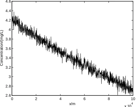
Stochastic factors were considered in the water quality model, so determinate solutions could not be given. So-lutions could only be represented in the form of the chastic process. We plotted the solutions with the sto-chastic process, as shown in Figure 4. In this study the
stochastic process was the white noise process with va-riance σ2 = 0.75.
From Figure 4 we can see that the water concentration
still showed an attenuated trend, while the concentration would fluctuate around the expectation centered at each corresponding displacement x. The fluctuations had a certain range, with variance of σ2 = 0.75. The impact of
0 2 4 6 8 10
x 104 2.6
2.8 3 3.2 3.4 3.6 3.8 4 4.2 4.4 4.6
x/m
C
o
nce
nt
ra
ti
on/
(m
g
/L)
Figure 4. Solutions of water quality model with stochastic process.
stochastic factors on the water quality was uncertain, and it was difficult to describe it exactly and numerically. However, we made some reasonable assumptions for stochastic factors and dealt with them using some ma-thematical tools. Thus we could obtain solutions with a stochastic process.
3. Conclusions
The impacts of changes of various parameters and sto-chastic factors on the water quality model were analyzed and discussed. Preliminary conclusions were obtained as follows.
1) The values of Δk and E1 had the opposite sign. When the deviation of the degradation coefficient Δk increased, the concentration error E1 decreased numeri-cally at the corresponding displacement x. When Δk > 0, E1 < 0, and the value of Cs would decrease; when Δk < 0,
E1 > 0, and the value of Cs would increase. A 1% change
in the degradation coefficient would cause about 0.15% error in the solute concentration. The impacts of Δk on E1 decreased with increasing x.
2) When the deviation of initial concentration “ΔC0” increased, the errorof the model “E2” also increased at the corresponding displacement x. There was a positive linear correlation between E2 and ΔC0. To reduce the initial concentration at the pollution source is the most common and effective way to manage water quality. By reducing the initial concentration, the requirements of water quality could be achieved through the self-purifi- cation ability of the river itself.
3) Stochastic factors did not significantly affect the at-tenuation trend of water quality. However, because of the stochastic interference, the concentration of the solute would fluctuate around the expectation centered at each corresponding displacement x.
4. Acknowledgements
This work was supported by the National Natural Sci-ence Foundation of China (No. 41071322, 71031001).
REFERENCES
[1] R. Noori, M. S. Sabahi, A. R. Karbassi and A. Baghvand, “Multivariate Statistical Analysis of Surface Water Qual-ity Based on Correlations and Variations in the Data Set,”
Desalination, Vol. 260, No. 1-3, 2010, pp. 129-136. doi:10.1016/j.desal.2010.04.053
[2] H. Furumai, “Rainwater and Reclaimed Wastewater for Sustainable Urban Water Use,” Physics and Chemistry of the Earth, Vol. 33, 2008, pp. 340-346.
doi:10.1016/j.pce.2008.02.029
[image:6.595.64.283.535.707.2]Vol. 30, No. 11-16, 2005, pp. 762-766.
[4] Y. Z. Tao and L. Jiang, “Influence of Groundwater Dis-charge on Decay Process of Contamination Concentration in River Flow,” Journal of Hydraulic Engineering, Vol. 39, No. 2, 2008, pp. 245-249.
[5] D. D. Adrian and T. G. Sanders, “Oxygen Sag Equation for Second-Order BOD Decay,” Water Research, Vol. 32, No. 3, 1998, pp. 840-848.
doi:10.1016/S0043-1354(97)00259-5
[6] H. W. Streeter and E. B. Phelps, “A Study of the Pollu-tion and Natural PurificaPollu-tion of the Ohio River,” Public Health Service, Bulletin No. 146, Washington DC, 1925. [7] E. J. Theriault, “The Dissolved Oxygen Demand of
Pol-luted Waters,” Public Health Service, Bulletin 173, Washington DC, 1927.
[8] G. M. Fair, “The Dissolved Oxygen Sag—An Analysis,”
Sewage Works Journal, Vol. 11, 1939, p. 445.
[9] H. W. Streeter, “Measures of NATURAL Oxidation in polluted Streams. I. The Oxygen Demand Factor,” Sew-age Works Journal, Vol. 7, No. 2, 1935, p. 251.
[10] H. A. Thomas, “The Slope Method for Evaluating the Constants of the First-Stage Biochemical Oxygen De-mand Curve,” Sewage Works Journal, Vol. 9, 1937, pp. 425-430.
[11] H. A. Thomas, “The Pollution Load Capacity of Streams,”
Water Sewage Work,Vol. 95, No. 11, 1948, p. 409. [12] D. J. O’Connor, “Oxygen Balance of an Estuary,”
Trans-actions, ASCE, Vol. 126, 1961, pp. 556-611.
[13] J. W. Clark and W. Viessman, “Water Supply and Pollu-tion Control,” InternaPollu-tional Textbook Company, 1965, pp. 387-390.
[14] H. B. Braun and P. M. Berthouex, “Analysis of Lag Phase BOD Curves Using the Monod Equations,” Water Re-sources Research, Vol. 6, 1970, pp. 838-844.
doi:10.1029/WR006i003p00838
[15] L. Somlyody, M. Henze, L. Koncsos, W. Rauch, P. Rei-chert, P. Shanahan and P. Vanrolleghem, “River Quality Modelling: III. Future of the Art,” Water Science and Technology, Vol. 38, No. 11, 1998, pp. 253-260. doi:10.1016/S0273-1223(98)00662-3
[16] A. Drolc and J. Z. Koncan, “Calibration of QUAL2E Model for the Sava River (Slovenia),” Water Science and Technology, Vol. 40, No. 10, 1999, pp. 111-118. doi:10.1016/S0273-1223(99)00681-2
[17] S. Cammara and C. W. Randall, “The Qual II Model,”
Journal of Environmental Engineering, Vol. 110, No. 5, 1984, p. 993.
doi:10.1061/(ASCE)0733-9372(1984)110:5(993)
[18] F. D. Masch and Associates, “QUAL-I Simulation of Water Quality in Stream and Canals, Program Documen-tation and User’s Manual,” Texas Water Development Board. 1970.
[19] Water Resources Engineers, Inc., “Computer Program Documentation for the Stream Quality Model QUAL-II. Prepared for US Environmental Protection Agency,” System Analysis Branch, Washington DC, 1973.
[20] L. C. Brow and T. O. Barnwell, “Computer Program
Documentation for the Enhanced Stream Water Quality Model QUAL2E,” US Environmental Protection Agency, Athens, GA, EPA/600/3-85/065, 1985.
[21] R. Portielje, T. H. Jacobsen and K. S. Jensen, “Risk Analysis Using Stochastic Reliability Methods Applied to Two Cases of Deterministic Water Quality Models,” Wa-ter Research, Vol. 34, No. 1, 2000, pp.153-170. doi:10.1016/S0043-1354(99)00131-1
[22] Y. Icaga, “Fuzzy Evaluation of Water Quality Classifica-tion,” Ecological Indicators, Vol. 7, No. 3, 2007, pp. 710- 718. doi:10.1016/j.ecolind.2006.08.002
[23] P. S. Kunwar, A. Basant, A. Malik and G. Jain, “Artificial Neural Network Modeling of the River Water Quality—A Case Study,” Ecological Modeling, Vol. 220, No. 6, 2009, pp. 888-895.
[24] H. Cho, K. S. Sung and S. R. Ha, “A River Water Quality Management Model for Optimizing Regional Wastewater Treatment Using a Genetic Algorithm,” Journal of Envi-ronmental Management, Vol. 73, No. 3, 2004, pp. 229- 242. doi:10.1016/j.jenvman.2004.07.004
[25] H. G. Cheng, Z. F. Yang and C. W. Chan, “An Expert System for Decision Support of Municipal Water Pollu-tion Control,” Engineering Applications of Artificial In-telligence, Vol. 16, No. 2, 2003, pp. 159-166.
doi:10.1016/S0952-1976(03)00055-1
[26] H. H. Liao and U. S. Tim, “Interactive Water Quality Modeling within a GIS Environment. Computer,” Envi-ronment, and Urban Systems, Vol. 18, 1994, pp. 343-363. doi:10.1016/0198-9715(94)90016-7
[27] X. W. Zhang, F. Qin and J. F. Liu, “Method of Monitor-ing Surface Water Quality Based on Remote SensMonitor-ing in Miyun reservoir,” Proceedings Bioinformatics and Bio-medical Engineering 3rd International Conference, Bei-jing, 2009, pp. 1-4.
[28] H. Apel, N.G. Hung, H. Thoss and T. Schöne, “GPS Buoys for Stage Monitoring of Large Rivers,” Journal of Hydrology, Vol. 412-413, 2012, pp. 182-192.
doi:10.1016/j.jhydrol.2011.07.043
[29] M. Q. Feng, B. M. Zheng and X. D. Zhou, “Water Envi-ronment Simulation and Prediction,” Science Press, Bei-jing, 2009, 181-197.
[30] Z. Z. Peng, T. X. Yang and X. J. Liang, “Mathematical Model of Water Environment and Its Application,” Chemical Industry Press, Beijing, 2007, pp. 98-103. [31] State Environmental Protection Administration of China,
General Administration of Quality Supervision, Inspec-tion and Quarantine of China (GB38382-2002), “ronmental Quality Standards for Surface Water,” Envi-ronmental Science Press, Beijing, 2002.
[32] F. Boano, R. Revelli and L. Ridolfi, “Stochastic Modeling of DO and BOD Components in a Stream with Random Inputs,” Advances in Water Resources, Vol. 29, No. 9, 2006, pp. 1341-1350.
doi:10.1016/j.advwatres.2005.10.007
[33] R. Revelli and L. Ridolfi, “Stochastic Dynamics of BOD in a Stream with Random Inputs,” Advances in Water Resources, Vol. 27, No. 9, 2004, pp. 943-952.
[34] W. Li and Z. Shi, “Robust Estimation of Water Quality Model Parameters under Random Noise Disturbance,”
Journal of Hydraulic Engineering, Vol. 37, No. 6, 2006, pp. 687-693.