Fuzzy Modeling using Vector Quantization with Supervised Learning

Fuzzy Modeling using Vector Quantization with

Supervised Learning

Hirofumi Miyajima, Noritaka Shigei, and Hiromi Miyajima

Abstract—It is known that learning methods of fuzzy mod-eling using vector quantization (VQ) and steepest descend method (SDM) are superior in the number of rules to other methods using only SDM. There are many studies on how to realize high accuracy with a few rules. Many methods of learning all parameters using SDM are proposed after determining initial assignments of the antecedent part of fuzzy rules by VQ using only input information, and both input and output information of learning data. Further, in addition to these initial assignments, the method using initial assignment of weight parameters of the consequent part of fuzzy rules is also proposed. Most of them are learning methods with simplified fuzzy inference, and little has been discussed with TS (Takagi Sugeno) fuzzy inference model. On the other hand, VQ method with supervised learning that divides the input space into Voronoi diagram by VQ and approximates each partial region with a linear function is known. It is desired to apply the method to TS fuzzy modeling using VQ. In this paper, we propose new learning methods of TS fuzzy inference model using VQ. Especially, learning methods using VQ with the supervised learning are proposed. Numerical simulations for function approximation, classification and prediction problems are performed to show the performance of proposed methods.

Index Terms—Fuzzy Inference Systems, Vector Quantization, Neural Gas, Vector Quantization with Supervised Learning, Appearance Frequency.

I. INTRODUCTION

With increasing interest in Artificial Intelligence (AI), many studies have been done with Machine Learning (ML). With ML, the supervised method such as BP learning for Multi-Layer Perceptron (MLP), the unsupervised one such as K-means method, and the Reinforcement Learning (RL) are well known. The learning method (fuzzy modeling) of fuzzy inference model is one of supervised ones, and many studies are conducted [1], [2]. Although most of conventional methods are based on steepest descend method (SDM), the obvious drawbacks of them are its large time complexity and getting stuck in a shallow local minimum. Further, there are problems of difficulty dealing with high dimensional spaces. In order to overcome them, some novel methods have been developed, which 1) create fuzzy rules one by one starting from any number of rules, or delete fuzzy rules one by one starting from sufficiently large number of rules [3], 2) use GA (Genetic Algorithm) and PSO (Particle Swarm Optimization) to determine fuzzy systems [4], 3) use fuzzy inference systems composed of small number of input rule

Hirofumi Miyajima is with the Okayama University of Science, 1-1 Ridaicho, Kitaku, Okayama, 700-0005, Japan

e-mail: k3768085@kadai.jp.

Noritaka Shigei is with Kagoshima University e-mail: shigei@eee.kagoshima-u.ac.jp

Hiromi Miyajima is with Kagoshima University e-mail: miya@eee.kagoshima-u.ac.jp.

This work was supported in part by the JSPS KAKENHI GRANT NUMBER JP17K00170.

modules such as SIRMs (Single Input Rule Modules) and DIRMs (Double Input Rule Modules) methods [5], and 4) use self-organization map (SOM) or VQ to determine the initial assignment of learning parameters [6], [7]. Especially, in learning methods of fuzzy inference model using VQ, there are many studies on how to realize high accuracy with a few rules [8], [9]. Many methods learning all parameters by SDM are proposed after determining the initial assignment of parameters of the antecedent part of fuzzy rules by VQ using only input information, and both input and output information of learning data. Further, in addition to these initial assignments, some methods using initial assignment of weight parameters of the consequent part of fuzzy rules are also proposed [8], [9]. Almost all of these are learning methods for simplified fuzzy inference model, and little has been discussed with TS fuzzy inference model [10]. On the other hand, a VQ method with the supervised learning that divides the input space into Voronoi diagram by VQ and approximates each partial region with a linear function is known [11]. It is desired to apply the method to determine the initial assignment of the parameters of TS fuzzy inference model to reduce the number of fuzzy rules.

In this paper, we propose new learning methods of TS fuzzy inference model using VQ. Especially, learning meth-ods using VQ with the supervised learning are proposed. In Section II, conventional learning methods of TS fuzzy model and VQ are introduced. Further, VQ with the supervised learning is introduced. In Section III, new learning methods for TS fuzzy inference model using VQ are proposed. In Section IV, numerical simulations for function approxima-tion, classification and prediction problems are performed to show the performance of proposed methods.

Although the proposed learning methods employ NG (Neural Gas) as a method of VQ, they also employ other VQ methods as well. Further, similar discussions can be developed for learning models other than the fuzzy inference model.

II. PRELIMINARIES

A. The conventional TS and simplified fuzzy inference models

The conventional fuzzy inference model using SDM is de-scribed [1], [10]. LetZj ={1,· · ·, j}andZj∗={0,1,· · ·, j} for the positive integerj. Let Rbe the set of real numbers. Let x = (x1,· · ·, xm) and yr be input and output data, respectively, wherexi∈R for i ∈Zm andyr∈R. Then the rule of TS fuzzy inference model is expressed as

Ri : if x1 isMi1 and· · ·xjisMij· · · andxmis Mim

then y iswi0+wi1x1+· · ·+wilxl+· · ·+wimxm, (1)

part, andwilis the weight of the consequent part. The model is called TS (Takagi Sugeno) fuzzy inference model [10]. If

wil = 0 for l∈Zm, then the model is called the simplified fuzzy inference model [1].

A membership valueµiof the antecedent part for inputx is expressed as

µi= m ∏

j=1

Mij(xj). (2)

If Gaussian membership function is used, then Mij is expressed as follow:

Mij(xj) = exp (

−1 2

(

xj−cij

bij )2)

(3)

wherecij andbij denote the center and the width values of

Mij, respectively.

The outputy∗ of fuzzy inference is calculated as follows:

y∗= ∑n

i=1µi( ∑m

l=0wilxl) ∑n

i=1µi

(4)

wherex0= 1.

In order to construct the effective model, the conventional learning is introduced. The objective function E is deter-mined to evaluate the inference error between the desirable output yr _{and the inference output y}∗_.

In this section, we describe the conventional learning algorithm [1].

Let D = {(xp₁,· · ·, xp

m, yrp)|p ∈ ZP} and D∗ = {(xp₁,· · ·, xp

m)|p∈ZP}be the set of learning data and the set of input data ofD, respectively. The objective of learning is to minimize the following mean square error (MSE):

E = 1

P

P ∑

p=1

(y∗_p−yr_p)2. (5)

In order to minimize the objective function E, each parameter α ∈ {cij, bij, wil} is updated based on SDM as follows [1]:

α(t+ 1) =α(t)−Kα

∂E

∂α (6)

where t is iteration time and Kα is a constant. When the Gaussian membership function is used as the membership function, the following relation holds.

∂E ∂wil

= ∑nµi i=1µi

(y∗−yr)xl (7)

∂E ∂cij

= ∑nµi i=1µi

(y∗−yr)( m ∑

l=0

wilxl−y∗)

xj−cij

b2

ij (8)

∂E ∂bij

= ∑nµi i=1µi

(y∗−yr)( m ∑

l=0

wilxl−y∗)

(xj−cij)2

b3

ij (9)

wherex0= 1,i∈Zn,j∈Zm andl∈Zm∗.

The conventional learning algorithm for TS model is shown as follows [1], where θ andTmax are the threshold and the maximum number of learning, respectively. Note that the method is generative one, which creates fuzzy rules one by one starting from any number of rules. The method is called learning algorithm A.

Learning Algorithm A

Step A1 : The number of rulesnis set ton0. Lett= 1. Step A2 : The parameterscij,bij andwil are set randomly.

Step A3 : Letp= 1.

Step A4 : A data(xp₁,· · ·, xp

m, yrp)∈D is given.

Step A5 : From Eqs.(2) and (4), µi andy∗ are computed.

Step A6 : Parameterscij,bijandwilare updated by Eqs.(7), (8) and (9).

Step A7 : Ifp=P, then go to Step A8 and ifp < P, then go to Step A4 withp←p+ 1.

Step A8 : Let E(t)be inference error at step t calculated by Eq.(5). If E(t)> θ and t < Tmax, then go to Step A3 witht←t+ 1else ifE(t)≤θ, then the algorithm terminates.

Step A9 : If t > Tmax andE(t)> θ, then go to Step A2 withn←n+ 1andt= 1.

B. Neural gas and K-means methods

Vector quantization techniques encode a data space, e.g., a subspaceV⊆Rd_{, utilizing only a finite setU ={ui|i∈Zr}} of reference vectors (also called cluster centers), wheredand

rare positive integers.

Let the winner vectorui(v)be defined for any vectorv∈V as follows:

i(v) = arg min i∈Zr

||v−ui|| (10)

From the finite setU,V is partitioned as follows:

Vi={v∈V|||v−ui||≤||v−uj|| f or j∈Zr} (11)

The evaluation function for the partition is defined as follows:

E= ∑

ui∈U

∑

v∈V

hλ(ki(v,ui)) ∑

ul∈Uhλ(kl(v,ul))

||v−ui(v)||2 (12)

For neural gas method [11], the following method is used: Given an input data vector v, we determine the neighborhood-rankinguik for k∈Zr∗−1, being the reference

vector for which there arek vectorsuj with

||v−uj||<||v−uik|| (13)

If we denote the numberkassociated with each vectorui byki(v,ui), then the adaption step for adjusting theui’s is given by

△ui=εhλ(ki(v,ui))(v−ui) (14)

hλ(ki(v,ui)) = exp (−ki(v,ui)/λ)) (15)

ε=εint (

εf in

εint ) t

Tmax

where ε∈[0,1] and λ > 0. The number λ is called decay constant.

If λ→0, Eq.(14) becomes equivalent to the K-means method [11]. Otherwise, not only the winner ui0 but the second, third nearest reference vectorui1,ui2, · · · are also updated in learning.

Letp(v)be the probability distribution of data vectors for

V. Then, NG method is introduced as follows [11]:

Learning Algorithm B∗ (Neural Gas Method)

Step B∗1 : The initial values of reference vectors are set randomly. The learning coefficientsεintandεf inare set. Let

Step B∗2 : Let t= 1.

Step B∗3 : Give a data v∈V based on p(x) and neighborhood-rankingki(v,ui)is determined.

Step B∗4 : Each reference vector ui for i∈Zr is updated based on Eq.(14)

Step B∗5 : Ift≥Tmax, then the algorithm terminates and the setU ={ui|i∈Zr} of reference vectors for V is obtained. Otherwise go to Step B∗3 ast←t+ 1.

If the data distribution p(v) is not given in advance, a stochastic sequence of input data v(1),v(2),· · · which is based on p(v)is given.

By using Learning Algorithm B∗, the learning method of fuzzy systems is introduced as follows [8] : In this case, assume that the distribution of learning data D∗ is discrete uniform one. Letn0 be the initial number of rules andn= n0.

Learning Algorithm B (Learning of fuzzy inference system using NG)

Step B1 : For learning dataD∗, Learning Algorithm B∗ is performed, where|U|=n.

Step B2 : Each element of the set U is set to the center parametercof each fuzzy rule.

Let

bij= 1

mi ∑

xk∈Ci

(cij−xkj)2, (16)

whereCiandmiare the set of learning data belonging to the

i-th cluster and its number, respectively. Each initial value of wil is selected randomly. lett= 1.

Step B3 : The Steps A3 to A8 of learning algorithm A are performed.

Step B4 : If t≥Tmax and E(t) > θ, then go to Step B1 withn←n+ 1.

C. Adaptively local linear mapping

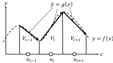
The aim in this section is to adaptively approximate the functiony=f(v)withv∈V⊆Rd _{andy∈Rusing VQ [11].} The setV denotes the function’s domain. Let us considern

computational units, each containing a reference vector ui together with a constant ai0 and d-dimensional vectors ai. Learning Algorithm B∗ assigns each unitito a subregionVi as defined in Eq.(11), and the coefficientsai0 andai define a linear mapping

g(v) =ai0+ai(v−ui) (17)

from Rd to R over each of the Voronoi diagram Vi (See Fig.1). Hence, the function y = f(v) is approximated by ˜

y=g(v) with

g(v) =ai(v)0+ai(v)(v−ui(v)) (18)

wherei(v)denotes uniti with itsui closest tov.

To learn the input-output mapping, a series of training steps by presenting D={(xp, y_pr)|p∈ZP} is performed. In order to obtain the output coefficientsai0 andai, the mean

squared error∑_v∈V (f(v)−g(v))2between the actual and the obtained output, averaged over subregion Vi, to be

Fig. 1. The concept of local linear mapping : The setViis one composed of

elementvclosest to the reference vectorui. The intervalViis approximated

by a local linear mapping.

minimal is required for each i. A gradient descent with respect toai0 andai yields [11].

△ai0=ε′hλ′(ki(v,ui))(y−ai0−ai(v−ui))(19)

△ai =ε′hλ′(ki(v,ui))(y−ai0−ai(v−ui))(v−ui)(20)

whereε′ >0andλ′>0.

The method means VQ with the supervised learning. The algorithm is introduced as follows [11] :

Learning Algorithm C

Input : Learning data D = {(xp_{, yp)|p∈Z}

P} and D∗ = {xp_|p∈Z

P}.

Output : The setU of reference vectors and the coefficients

ai0 andai for i∈Zn.

Step C1 : The set U of reference vectors is determined using D∗ by Algorithm B∗. The subregionsVi for i∈Zn is determined usingU, whereVi is defined by Eq.(11), Vd = ∪r

i=1Vi andVi∩Vj=∅ (i̸=j).

Step C2 : Parameters ai0 and ai are set randomly. Let

t= 1.

Step C3 : A learning data (x, y)∈D is selected based on

p(x). The rankki(x,ui)of xfor the setVi is determined.

Step C4 : Parametersai0andaifori∈Zrare updated based on Eqs.(19) and (20).

Step C5 : Ift≥Tmax, then the algorithm terminates else go to Step C3 witht←t+ 1.

Remark that Algorithm C is one of learning methods using NG and SDM [11].

D. The appearance frequency of learning data based on the rate of change of output

Learning Algorithm B is a method that determines the initial assignment of fuzzy rules by vector quantization using the set D∗. In this case, the set of output in learning data

D is not used to determine the initial assignment of fuzzy rules. In the previous paper, we proposed a method using both input and output data to determine the initial assignment of parameters of the antecedent part of fuzzy rules [8].

Based on Ref. [8], the appearance frequency is defined as follows : LetD andD∗ be the sets of learning data defined in Section 2.1.

Algorithm for Appearance Frequency (Algorithm AF) Step 1 : Give an input data xi∈D∗, we determine the neighborhood-ranking (xi0_,xi1_,· · ·_,xik_,· · ·_,xiP−1_{) of the} vector xi with xi0 _{= x}i_{, x}i1 _{being closest to x}i _and

xik_{(k = 0,}· · ·_{, P} −_{1) being the vector x}i _{for which there}

arek vectorsxj with||xi−xj||<||xi−xik||_.

of inclination of the output around output data to input data

xi_{, by the following equation:}

H(xi) = M ∑

l=1

|yi−yil|

||xi−_xil|| (21)

where xil _{for l}∈_Z

M means the l-th neighborhood-ranking of xi_,i∈Z

P andyi andyil are output for input xi andxil, respectively. The number M means the range considering

H(x).

Step 3 : Determine the appearance frequency (probability)

pM(xi)forxi by normalizing H(xi).

pM(xi) =

H(xi₎ ∑P

j=1H(xj)

(22)

The method is called Algorithm AF.

Learning algorithm D using Algorithm AF to TS fuzzy modeling is obtained as follows:

Learning Algorithm D Step D1 : The constantsθ,T0

max,TmaxandM0 for1≤M0

are set. Let M =M0. The probabilitypM(x)for x∈D∗ is computed using Algorithm AF. The initial numbernof rules is set.

Step D2 : The initial values of cij, bij and wil are set randomly.

Step D3 : Select a data(xp_{, yp)based onp} M(x).

Step D4 : Update cij by Eq.(14).

Step D5 : If t < T_max0 , go to Step D3 with t←t+ 1, otherwise go to Step D6 with t←1.

Step D6 : Determine bij by Eq.(16).

Step D7 : Letp= 1.

Step D8 : Given a data(xp_{, y}r p)∈D.

Step D9 : Calculate µi andy∗ by Eqs.(2) and (4).

Step D10 : Update parameterswil,cij andbij by Eqs.(7), (8) and (9).

Step D11 : Ifp < P then go to Step D8 withp←p+ 1.

Step D12 : If E > θ and t < Tmax then go to Step D8 witht←t+ 1, whereE is computed as Eq.(5), and ifE < θ

then the algorithm terminate, otherwise go to Step D2 with

n←n+ 1.

As shown in Ref. [8], learning algorithm D realizes that many rules are needed at or near the places where output changes rapidly in learning data. The probability pM(x) is one method to perform it [8]. See the Ref. [8] about the detailed explanation of Algorithms AF and D for the simplified fuzzy modeling.

III. PROPOSED METHODS OFTSFUZZY MODELING USINGVQ

It is known that learning methods for the simplified fuzzy model using VQ and SDM are effective in accuracy and the number of rules compared to other methods using only SDM. Further, it is also known that TS fuzzy inference model is superior in accuracy to the simplified fuzzy inference model [10]. Then, how is the performance of TS fuzzy modeling using VQ? The conventional methods learning all parameters in SDL is easily applied to TS fuzzy modeling after determining initial assignments of the antecedent part of fuzzy rules by VQ using only input information, and both input and output information of learning data (See the

Fig. 2. The concept of Algorithm E

methods B and C). However, learning methods with weight parameters of the consequent part are difficult to apply to TS Fuzzy inference model. Therefore, we propose new learning methods using the Learning Algorithm C as follows:

Learning Algorithm E

Input : Learning data D = {(xp_{, yp)| p∈Z}

P} and D∗ = {xp_|p∈Z

P}.

Output : Parametersc,bandwof TS fuzzy inference model.

Step E1 : From Algorithm AF, the probability pM(x) is computed usingD.

Step E2 : From Algorithm B∗, the setUof reference vectors is computed usingpM(x).

Step E3 : From Algorithm C, parameters ai0 and ai of local linear mapping are computed using the setU.

Step E4 : Each element of the set U is set to the center parametercof each fuzzy rule and the widthbof each fuzzy rule is computed from Eq.(19). Parametersai0andaiof local linear mapping are set to the initial parameters of wi0 and wi for fuzzy rules.

Step E5 : Let t = 1. Parametersc, b andw are updated from Step A3 to A8 of Algorithm A.

Step E6 : If t > Tmax andE(t)> θ1, then go to Step E2 withn←n+ 1as adding a fuzzy rule.

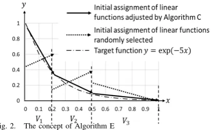
Let us explain Algorithm E using an example. [Example]

The problem is that approximates the function y = exp(−5x) using ten learning data shown in Table I, where

D∗={0.1×k|k∈Z₁₀∗ } andD={(x,exp(−5x))|x∈D∗}. From Step E1, a probabilitypM(x)is formed as shown in Table I, where the numberrof reference vectors is 3.

From Step E2, VQ is performed based on pM(x). Let

M = 3. For example, two reference vectors are assigned in the interval from 0 to 0.4, and one reference vector is assigned for the remaining interval. Three regions V1, V2

andV3 shown in Fig.2 are defined as Voronoi regions from

the set U of reference vectors.

From Step E3, a linear function is defined in each region. In the example, interval linear functions as shown in Fig.2 are obtained as the result of learning. If algorithm C is not used, each linear function is given randomly as shown in Fig.2.

From Steps E2 and E3, the initial parameters of the antecedent and the consequent parts of fuzzy rules are determined, respectively.

TABLE I

LEARNING DATA FOREXAMPLE OFy= exp(−5x)

In order to compare the proposed methods with conven-tional ones, the following learning methods for TS model are used (See Fig.3):

(A) The method A is Learning Algorithm A, that is the con-ventional learning method for TS model. Initial parameters of

c,bandw are set randomly and all parameters are updated using SDM until the inference error becomes sufficiently small.

(B) The method B is generalized one of learning method of RBF networks [1]. Initial values of c are determined using the setD∗ by VQ andbis computed usingc. Weight parametersware randomly selected. Further, all parameters are updated using SDM until the inference error becomes sufficiently small.

(B’) The method B’ is the proposed one. In addition to the initial assignment of the method B, the initial assignment of weight parameters of the consequent part is determined by Algorithm C. Further, all parameters are updated using SDM until the inference error becomes sufficiently small.

(C) The method C is Learning Algorithm D. Initial values of

care determined using the setD by VQ andbis computed using c. Weight parameters are randomly selected. Further, all parameters are updated using SDM until the inference error becomes sufficiently small.

(C’) The method C’ is the Algorithm E. In addition to initial assignment of the method C, the initial assignment of weight parameters of the consequent part is determined by the Algorithm C. Further, all parameters are updated using SDM until the inference error becomes sufficiently small.

IV. NUMERICAL SIMULATIONS

In order to show the effectiveness of the proposed meth-ods, simulations of function approximation, classification and prediction problems are performed.

A. Function approximation

In order to show the effectiveness of proposed meth-ods, numerical simulations of function approximation are performed. The systems are identified by fuzzy inference systems. This simulation uses three systems specified by the following functions with 2 and 4-dimensional input space [0,1]2 (Eq.(23)) and [−1,1]4 (Eqs.(24) and (25)), and one output with the range [0,1]. The number of Learning and Test data are 500 and 1000 for Eq.(23) and 512 and 6400

Fig. 3. Concept of conventional and proposed algorithms, where SDM andd NG mean Steepest Descent Method and Neural Gas method and the feedback loop means the adding of fuzzy rules.

TABLE II

THE RESULTS FOR FUNCTION APPROXIMATION

Eq(23) Eq(24) Eq(25) the number of rules 4.9 4.2 3.0 A MSE for Learning(×10−4_{) 0.37 0.31 0.20}

MSE of Test(×10−4_{) 0.49 0.46 0.22}

the number of rules 4.1 4.0 3.0 B MSE of Learning(×10−4_{) 0.26 0.42 0.19}

MSE of Test(×10−4_{) 0.32 0.56 0.22}

the number of rules 4.1 4.1 3.1 B’ MSE of Learning(×10−4_{) 0.26 0.49 0.21}

MSE of Test(×10−4_{) 0.32 0.68 0.25}

the number of rules 4.4 4.1 3.1 C MSE of Learning(×10−4_{) 0.29 0.49 0.21}

MSE of Test(×10−4_{) 0.47 0.68 0.25}

the number of rules 4.1 4.1 3.0 C’ MSE of Learning(×10−4_{) 0.26 0.54 0.18}

MSE of Test(×10−4_{) 0.35 0.76 0.21}

for Eqs.(24) and (25), respectively.

y = sin(10(x1−0.5)

2_{+ 10(x2−0.5)}2_{) + 1}

2 (23)

y = (2x1+ 4x

2 2+ 0.1)2

74.42

+(3e

3x3_{+ 2e}−4x4₎−0.5−_0.077

4.68 (24)

y = (2x1+ 4x

2 2+ 0.1)2

74.42

×(4 sin(πx3) + 2 cos(πx4) + 6)

446.52 (25)

The constantsθ,Tmax,Kcij,Kbij andKwi for each

algo-rithm are1.0×10−4_{,50000,0.01,0.01and0.1, respectively.}

The constantsεinit,εf inandλfor Algorithms B, B’, C and C’ are 0.1, 0.01 and 0.7, respectively. The constants ε′_init,

ε′_{f in}andλ′ for Algorithms B’ and C’ are0.1,0.01and0.7, respectively.

TABLE III

THE DATASET FOR PATTERN CLASSIFICATION

Iris Wine BCW Sonar The number of data 150 178 683 208 The number of input 4 13 9 60 The number of class 3 3 2 2

TABLE IV

THE RESULT FOR PATTERN CLASSIFICATION

Iris Wine BCW Sonar the number of rules 2.2 2.2 2.1 3.2 A RM for Learning(%) 2.8 1.6 2.4 0.4 RM of Test(%) 3.5 6.1 3.8 19.4 the number of rules 2.1 2.1 2.4 5.6 B RM of Learning(%) 3.0 1.5 2.4 0.4 RM of Test(%) 4.5 6.1 3.9 22.6 the number of rules 2.2 2.1 2.2 5.4 B’ RM of Learning(%) 3.0 1.5 2.4 0.4 RM of Test(%) 4.3 5.9 3.8 21.8 the number of rules 2.2 2.1 2.2 2.7 C RM of Learning(%) 3.0 1.5 2.4 0.2 RM of Test(%) 4.3 5.9 3.8 24.3 the number of rules 2.0 2.0 2.0 2.8 C’ RM of Learning(%) 2.6 1.5 2.5 0.1 RM of Test(%) 4.3 4.4 3.9 23.5

B. Classification problems

Iris, Wine, BCW and Sonar data from UCI database shown in Table III are used for numerical simulation [12]. In this simulation, 5-fold cross-validation is used as the evaluation method. Threshold θ is 0.01 on Iris and Wine and 0.02 on BCW and Sonar, respectively.Tmax,Kcij,Kbij andKwifor

each algorithm are 50000, 0.01, 0.01 and 0.1, respectively.

εinit, εf in andλ for Algorithms B, C, B’ and C’ are 0.1, 0.01and0.7, respectively.ε_init′ ,ε′_{f in}andλ′ for Algorithms B’ and C’ are 0.1,0.01and0.7, respectively.

Table IV shows the result of classification for each al-gorithm, where the number of rules means one when the thresholdθof inference error is achieved in learning. In Table IV, the number of rules and RM’s for learning and test are shown, where RM means the rate of misclassification. The result of simulation is the average value from twenty trials. It is shown that the proposed method C’ is superior in the number of rules to conventional methods.

C. Prediction of the Mackey-Glass Time Series

In this section, the prediction problem of time series generated by the Mackey-Glass equation is performed [11]. The prediction one requires to learn an input-output function

y = f(v) of a current state v of the time sequences into prediction of a future time series value y.

The Mackey-Glass equation is represented as follows :

∂x(t)

∂t =βx(t) +

αx(t−τ)

1 +x(t−τ)10 (26)

whereα= 0.2,β =−0.1andτ = 17.x(t)is qusi-periodic and chaotic with a fractal attractor dimension 2.1 for the parameters.

In this simulation, let training pairs v = (x(t), x(t −

6), x(t−12), x(t−18), y=x(t+6)), that is, 4 inputs and one output. The numbers of learning and test data are 1000 and 1000, generated by Eq.(26), respectively. After learning using 1000 data, data of 1000 steps are predicted. The function is identified by fuzzy inference systems. θ,Tmax,Kcij, Kbij

andKwifor each algorithm are1.0×10−

5_{,50000,0.01,0.01}

and0.1, respectively.εinit,εf inandλfor Algorithms B, B’,

TABLE V

THE RESULT FOR FUNCTION APPROXIMATION

A B B’ C C’

the number of rules 9.6 6.1 5.8 5.0 5.1 MSE of Learning(×10−5_{) 0.83 0.85 0.80 0.84 0.77}

MSE of Test 0.103 0.103 0.102 0.103 0.103

C and C’ are0.1,0.01and0.7, respectively.ε′_init,ε′_{f in}andλ′

for Algorithms B’ and C’ are0.1,0.01and0.7, respectively. The result of simulation is shown in Table V. The result of simulation is the average value from twenty trials. The result of Table V shows that proposed methods are in the number of rules superior to conventional ones.

V. CONCLUSION

In this paper, we proposed new learning methods of TS fuzzy inference model using VQ. Especially, learning meth-ods using VQ with the supervised learning were proposed. With TS fuzzy modeling, conventional methods learning all parameters in SDL were proposed after determining initial assignments of the antecedent part of fuzzy rules by VQ using only input information, and both input and output information of learning data. In addition to these initial assignments, the methods determining weight parameters of linear functions of the consequent part of fuzzy rules were proposed. In numerical simulations for function approx-imation, classification and prediction problems, proposed methods were superior in the number of rules to conventional ones.

In the future work, other learning methods using VQ in TS fuzzy modeling will be proposed and other SDM methods using VQ with the supervised learning will be considered.

REFERENCES

[1] M.M. Gupta, L. Jin and N. Homma, Static and Dynamic Neural Networks, IEEE Press, 2003.

[2] J. Casillas, O. Cordon, F. Herrera and L. Magdalena, Accuracy Improvements in Linguistic Fuzzy Modeling, Studies in Fuzziness and Soft Computing, Vol. 129, Springer, 2003.

[3] S. Fukumoto, H. Miyajima, K. Kishida and Y. Nagasawa, A Destruc-tive Learning Method of Fuzzy Inference Rules, Proc. of IEEE on Fuzzy Systems, pp.687-694, 1995.

[4] O. Cordon, A historical review of evolutionary learning methods for Mamdani-type fuzzy rule-based systems, Designing interpretable genetic fuzzy systems, Journal of Approximate Reasoning, 52, pp.894-913, 2011.

[5] H. Miyajima, N. Shigei and H. Miyajima, Fuzzy Inference Systems Composed of Double-Input Rule Modules for Obstacle Avoidance Problems, IAENG International Hournal of Computer Science, Vol. 41, Issue 4, pp.222-230, 2014.

[6] K. Kishida and H. Miyajima, A Learning Method of Fuzzy Inference Rules using Vector Quantization, Proc. of the Int. Conf. on Artificial Neural Networks, Vol.2, pp.827-832, 1998.

[7] S. Fukumoto, H. Miyajima, N. Shigei and K. Uchikoba, A Decision Procedure of the Initial Values of Fuzzy Inference System Using Counterpropagation Networks, Journal of Signal Processing, Vol.9, No.4, pp.335-342, 2005.

[8] H. Miyajima, N. Shigei and H. Miyajima, Fuzzy Modeling using Vector Quantization based on Input and Output Learning Data, Inter-national MultiConference of Engineers and Computer Scientists 2017, Vol.I, pp.1-6, Hong Kong, March, 2017.

[9] W. Pedrycz, H. Izakian, Cluster-Centric Fuzzy Modeling, IEEE Trans. on Fuzzy Systems, Vol. 22, Issue 6, pp. 1585-1597, 2014.

[10] T. Takagi, M. Sugeno, Fuzzy identification of systems and its appli-cations to modeling and control, IEEE Trans. on Systems, Man, and Cybernetics, Vol.SMC-15, No.1, pp.116-132, 1985.

[11] T. M. Martinetz, S. G. Berkovich and K. J. Schulten, Neural Gas Network for Vector Quantization and its Application to Time-series Prediction, IEEE Trans. Neural Network, 4, 4, pp.558-569, 1993. [12] UCI Repository of Machine Learning Databases and Domain Theories,