SOFT Development of feature tracking methods

SOFT

Satellite-Based Ocean Forecasting

EVK3-CT-2000-00028

Coordinator: Dr. Joaquín Tintoré

Progress Report

WP 3 – Task 3.1

Development of feature tracking methods

January 2003

Paolo Cipollini, Peter Challenor

Southampton Oceanography Centre, U.K.

Introduction

The present report describes the work carried out within task 3.1 of Work Package 3 of the SOFT Project (hereinafter simply ‘the Project’). The above task is ‘Development of feature tracking methods’ and consists of the development of a software to track large-scale, westward propagating features (planetary waves or westward-travelling eddies) in the altimetric datasets, and in the removal of the identified features from the datasets. The residual field (that is the original dataset minus the tracked features) is then made available to the other work packages in the Project.

Rationale

A significant part of mid-latitude oceanic variability at meso- to large-scale (scales > 100 km) consists of features or disturbances propagating westward with speeds of the order of few cm/s and amplitudes of a few cm in the sea surface height (SSH) field; these features are westward-propagating eddies or mid-latitude baroclinic planetary waves (Chelton and Schlax, 1996, Fu and Chelton, 2001). The existence of planetary waves in the oceans had been accepted in view the theory developed by Carl-Gustav Rossby in the 1930s, but it is only with the advent of satellite altimetry in the 1990s that these features have been directly observed and their properties studied (for a review, see Cipollini et al., 2000). They have important effects on the circulation and on the structure of the ocean at depth. Moreover, they have been observed recently in the global sea surface temperature dataset (Hill et al., 2000) and in the global ocean colour dataset (Cipollini et al, 2001; Uz et al., 2001)

So far all the studies of westward-propagating disturbances in the oceans have been carried out with techniques that infer the average properties of the disturbance field over an extended spatio-temporal domain. The only exceptions are those works dealing with the discrete tracking of eddy-like structures -- however these exercises usually cover a very limited time and space frame. As a consequence we have some idea of the mean properties (surface amplitude, period or time scale, wavelength or spatial scale, speed) of the propagating features, but without the degree of geographical detail that can be obtained from theoretical predictions (Killworth and Blundell, 2003a,b). Moreover, until now we have not been able to predict how a disturbance would evolve on the basis of its present location and characteristics (for instance, we are still unable to say that a planetary wave at location x1 with a speed v1

would ‘most likely’ have a speed v2 at location x1+∆t v1) if not on the basis of average,

low-pass statistics of the propagation field (like those that can be inferred by standard analysis methods such as the spectral analysis of longitude/time plots). If we were able to study the evolving characteristics of every single propagating disturbance, it would then be possible to build an archive of the characteristics; and finally, we would be able to predict the behaviour of any new propagating event on the basis of the behaviour of past events recorded in the archive. But all the above requires a change of approach –a transition from ‘averaging’ methods like Fourier transforms to methods trying to identify and study the single disturbance events (like well-identifiable solitons, as opposed to a periodic wave field).

behaviour of any new propagating event, is exactly the overall purpose of Work Package 3 in the SOFT Project. The present report covers the first part of the work (task 3.1), that is the methodology for the identification (tracking) of the single features in the satellite datasets (sea surface height), and its application to SSH data in the Azores region in the North Atlantic. This is a highly energetic region where previous studies have identified a number of propagating features (see for instance Cipollini et al., 1999, Cromwell, 2001)

Task 3.1 has two main outcomes:

a) the tracked features are removed from the datasets, and the residual fields are passed to other packages (like Work Package 2) for the testing of the non-linear time series predictors;

b) the archive of propagation characteristics is passed on to task 3.2 in order to forecast the evolution of any new propagating disturbance; the predicted field will then be recombined to the forecasts of the non-linear predictors mentioned in a) to give a SOFT hybrid forecast of the height field.

Methodology and Results

SSH data preconditioning

For the analysis we use TOPEX/Poseidon SSH anomalies, calculated with respect to the 1993-1995 mean at each location along the satellite ground track, and gridded on a 1° x 1° x 1 orbital cycle grid (1 orbital cycle=9.9156 days). These data are part of the GADGET archive of gridded satellite data at SOC, and are available both in MATLAB and NetCDF format. The full mid-latitude North Atlantic dataset has been made available to all the SOFT partners, alongside chlorophyll concentration data from SeaWiFS and SST data from AVHRR.

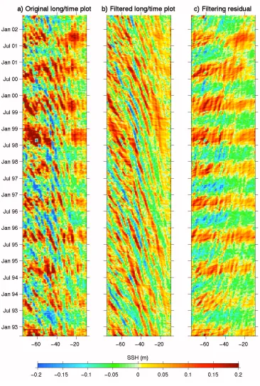
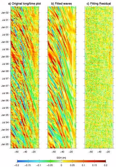
In our analysis we covered the region 20°N to 40°N and 75°W to 8°W, which we refer to in the following as ‘the study area’. At any given latitude we first extracted the longitude/time section of the data (covering the entire longitude section, except for any land on the sides). As an example to illustrate the data processing we will use 34°N, given that the propagation characteristics at that latitude are well documented (Cromwell, 2001). Figure 1a shows the longitude/time plot at 34°N prior to any data processing. The plot shows clear westward-propagating signals (most likely to be planetary waves) as slanted alignments of positive and negative anomalies. The annual cycle is also apparent in figure 1a.

The longitude-time plot at any latitude was filtered with a westward-only filter, that is a filter that in the wavenumber/frequency space (that is the 2-D Fourier Transform of the longitude/time space) removes the quadrants containing the eastward propagation. It also removes the two axis wavenumber=0 (thus cutting most of the annual signal) and frequency=0 (thus removing any stationary signal). To improve the removal of the annual component, a 3 x 3 cluster of spectral bins around the annual peak was also removed in the wavenumber/frequency space. Figure 1b shows the filtered longitude/time plot and figure 1c shows the filtering residual, which contains both the annual signal and any eastward-propagating component, and which is available to the Project partners on the FTP site (this may eventually be recombined with the fitting residuals described below, prior to the forecasts of Work Package 2)

Wave model fitting

The approach followed to identify the single waves at any given latitude can be summarized as follows:

a) split the full longitude/time plot into a number of overlapping sub-windows

b)for each sub-window, fit a number of elementary waves by minimizing the mean square error with respect to a wave shape model

c) reconstruct the trajectories of any single wave event by ‘joining’ the elementary waves in a sub-window with those in the adjacent window to the west

a) Extraction of the sub-windows

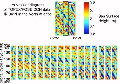
To ensure that the fitting yields the ‘local’ properties of the propagating disturbances, the filtered longitude/time plot is split into a number of overlapping sub-windows, which can be thought of as subsetting the dataset by means of a window of width Λ degrees and moving by ∆λ degrees at each step. Figure 2 shows this concept on a test dataset; the overlap between adjacent windows is apparent. For the analysis we used Λ=11 degrees and ∆λ=1 degree. These values were selected somewhat empirically as a trade-off between localization of the features and statistical robustness of the fitting procedure. As a consequence, any sub-window overlaps its immediate neighbour by almost 90%, thus ensuring that the longitudinal variation of the parameters can be estimated in detail. To further improve the fitting and the localization of the features we multiplied (tapered) any sub-window by a raised cosine profile (11-point hanning window) in longitude, so that the centre point in longitude is multiplied by a unit weight and the weight decreases towards each side of the sub-window.

Figure 2 – Example of subsetting af a longitude/time plot into partially overlapping sub-windows

b) Fitting the wave model

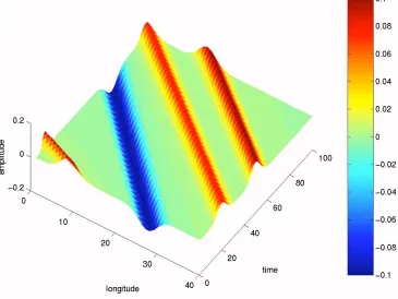
Figure 3 – sum of four 2-D gaussian shapes

G=Aexp(−

x− t s−p

(

)

2σ2 )

where x is longitude and t time. Figure 3 shows a 3-D representation of the sum of 4 gaussian shapes (3 ‘crests’ and 1 ‘trough’) in a longitude/time space. Each one of those features is described by the 4 parameters(A, s, p, σ). Parameters s and p

are the slope and x-intercept of the line t=s(x-p) representing the track of the propagating feature on the plot; the slope s is thus linked to the speed of the feature. Parameter σ gives the horizontal (zonal) scale of the feature. Given that we use tapered subsets of data, in the fitting code we actually fitted tapered gaussians (with the same 11-point hanning window) to the data. Tapering does improve the estimation of the local amplitude of the features (i.e. the amplitude near the longitudinal centre of the sub-window, which may differ from the ‘mean’ amplitude of a non-tapered feature).

The actual fitting is done with a Levenberg-Marquardt mean square error minimization algorithm (using the MATLAB function lsqcurvefit), which obviously needs a quadruplet of parameters (A₀, s₀, p₀, σ₀) as a starting point. In our fitting scheme |A0| is set to 10 cm, σ0 to 1 degree and the other two parameters are

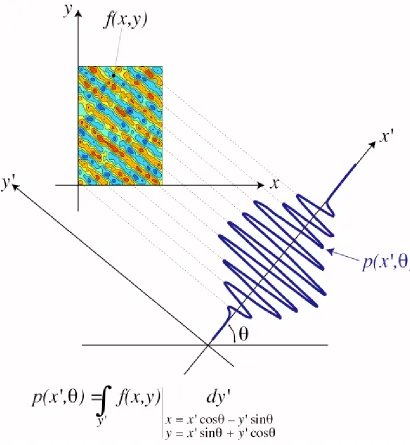
processing for its ability to find alignments in the dataset, and as such has been used in satellite oceanography to estimate the speed of planetary waves (Chelton and Schlax, 1996, Cipollini et al., 1999, Hill et al., 2000, Cipollini et al., 2001, Challenor et al., 2001). Here we find the maximum of the absolute value of the RT of the tapered sub-window and from its position (x’max,θmax) in the RT space we compute the

initial estimate s₀, p₀ for the intercept and slope of the feature (crest or through) in the plot. The sign of the peak in the RT also tells us the sign of A₀.

Figure 4 – Definition of the Radon Transform

for the observed scatter in the speed of planetary waves (Fu and Chelton, 2001), and ensures that only well-understood propagating features are actually fitted to the data.

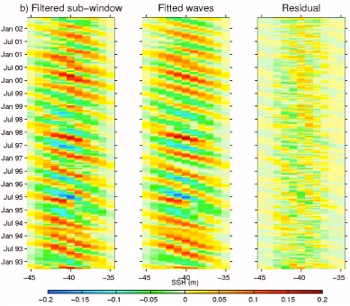
The tapered gaussian whose initial slope and intercept correspond to the strongest peak in the RT is fitted first; then that elementary wave is removed from the tapered sub-window, and the fitting is iterated over the residual. When for a particular set of initial conditions the fitting algorithm either does not converge, or converges on a gaussian whose amplitude is below a threshold, the search is moved to the next largest peak in abs(RT). As amplitude threshold we used the largest between 2.5 cm and 0.8 times the standard deviation of the residual. This ensures that the largest amplitude features are fitted first. The iterative search exits (and moves to the next sub-window) when an acceptable solution cannot be found in the 5 largest peaks of abs(RT). Figure 5 illustrates the fitting process with an example centred at 34 N, 40W.

Figure 5 – example of fitting of elementary waves on a 11° tapered sub-window: a: filtered and tapered sub-window; b) field of the fitted waves; c) residuals

longitude/plot. Figure 7 shows the standard deviation of the filtered longitude/plot and of the compacted fitted wave and residual fields at each latitude.

Figure 7 – Standard deviation in the filtered longitude/time plot, fitted wave field and residual field

The compacted residuals have been provided to the other Project partners for use into other work packages (like Work Package 2 for the testing of the non-linear time series predictors). Their forecasts will then be merged with the forecasted propagation of the single wave events (which are identified as explained below) to be carried out in Work Package 3.2; the result will be the implementation of a hybrid SOFT tracking method.

c) Reconstruction of the single wave events

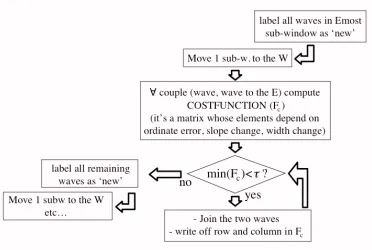
the east, and write off the relevant row and column in the matrix so that the two waves cannot be joined to any others. Once all the minima below the cost threshold in F_c have been accounted for, we label all the remaining waves as ‘new’ and move to the next sub-window to the west, and so on. The result is in the form of a MATLAB data structure, that is a structured table where any entry represents a ‘joined’ wave (that is, a single wave event made by one or more elementary waves), and lists the evolution of its parameters with longitude.

Figure 8 - Flow diagram of the program joining the elementary waves

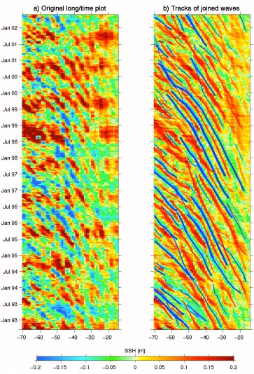
Figure 9 – a) original longitude/time plot at 34N; b) tracks of those joined waves (single wave events) which propagate for at least 5° in longitude, superimposed on the

Figure 10: a) median amplitude of those waves at 34°N which propagate for at least 5° in longitude; b) median speed; c) median width.

event(s) in the past, by defining an appropriate distance in the parameter space. It is worth to note that such an approach for the forecast is only made possible by the fact that we have been able to identify the evolution of any single wave crest and through in the dataset, by means of the model-fitting analysis and subsequent ‘joining’ of the waves.

References

Challenor, P. G., P. Cipollini and D. Cromwell, “Use of the 3-D Radon Transform to examine the properties of oceanic Rossby waves”, Journal of Atmospheric and Oceanic Technology, vol. 18, no. 9, pp. 1558-1566, 2001 – see also:

“Corrigendum”, Journal of Atmospheric and Oceanic Technology, vol. 19, no. 5, p. 828, 2002.

Chelton, D. B. and M. G. Schlax, Global observations of oceanic Rossby waves,

Science, 272, 234-238, 1996.

Cipollini, P., D. Cromwell, G. D. Quartly and P. G. Challenor, “Remote Sensing of oceanic extra-tropical Rossby waves”, Satellites, Oceanography and Society, edited by David Halpern, ch. 6, pp. 99-123, Elsevier Science Ltd, 2000. (Elsevier

Oceanography Series, 63).

Cipollini, P., D. Cromwell and G. D. Quartly, Observations of Rossby Wave propagation in the Northeast Atlantic with TOPEX/POSEIDON altimetry, Adv. Space Res., 22, 1553-1556, 1999.

Cipollini, P., D. Cromwell, P. G. Challenor and S. Raffaglio, “Rossby waves detected in global ocean colour data”, Geophysical Research Letters, Vol. 28 , No. 2 , pp. 323-326, 2001.

Cromwell, D. 2001: Sea surface height observations of the 34°N ’waveguide’ in the North Atlantic Geophys. Res. Lett., 28, 19, 3705-3708

Deans, S.R., The Radon transform and some of its applications, John Wiley and Sons, New York, 1983.

Fu, L.-L. and D. B. Chelton, Large Scale Ocean circulation, in Satellite Altimetry and

Earth sciences, eds. L.-L. Fu and A. Cazenave, Academic Press, 2001.

Hill, K. L., I. S. Robinson, and P. Cipollini, “Propagation characteristics of

extratropical planetary waves observed in the ATSR global sea surface temperature record”, Journal of Geophysical Research - Oceans, v. 105(C9), pp. 21,927-21.945, 2000.

Killworth, P. D. and J. R. Blundell, 2003a: Long extra-tropical planetary wave propagation in the presence of slowly varying mean flow and bottom topography. I: the local problem. J. Phys. Oceanogr., in press.

Killworth, P. D. and J. R. Blundell, 2003b: Long extra-tropical planetary wave

propagation in the presence of slowly varying mean flow and bottom topography. II: ray propagation and comparison with observations. J. Phys. Oceanogr., in press. Uz, B. M., Yoder, J. A. & Osychny, V. Pumping of nutrients to ocean surface waters