clearing methods for single-cell phenotyping in
whole organs
Thesis by
Ken Yee Chan
In Partial Fulfillment of the Requirements for the degree of
Doctor of Philosophy
CALIFORNIA INSTITUTE OF TECHNOLOGY Pasadena, California
2017
2017 Ken Yee Chan
ACKNOWLEDGMENTS
I begin by thanking my Ph.D. advisor, Dr. Viviana Gradinaru, for her guidance, hard work, dedication, persistence, and patience over the course of my Ph.D. training. Throughout my training, Viviana has advised me a great deal both professionally and personally. Viviana sets the bar high for each of her mentees, but because of her hard work, calm and caring nature, and dedication, she has provided me with the necessary means to achieve my goals during my Ph.D. training. She has done this by providing invaluable guidance and advice, an uncanny amount of resources, and a positive lab environment for learning, individual growth, and collaboration. Her patience and guidance has allowed me to learn many of the most up-to-date techniques in neuroscience, as well as valuable off-the-bench skills, such as writing papers, grants, and abstracts for conferences. She has also nurtured my future career by providing me with opportunities in presenting my work at numerous conferences and also allowing me to participate in many collaborations with other top scientists around the country. I am convinced my journey as a graduate student would not have been as productive and eventful had Viviana not taken the chance on accepting me into her lab. I hope her journey in mentoring me has been as positive and enjoyable as much as it has been for me in being her graduate student.
There are a few people without whom much of the work presented in this thesis would not have been possible, including my colleague and dear friend Dr. Alon Greenbaum. I have worked closely with Alon on many projects and have enjoyed and appreciated his candor and determination in getting things done. Alon’s need for perfection, consistency, and efficiency has been a major backbone in our work together. I feel very fortunate to have worked alongside Alon on our projects. One of the most important things I have learned from Alon was how to carry out a project and finish it. I have always felt fortunate to have been paired with Alon and would never want to miss an opportunity to work alongside him, if possible.
I would also like to thank a few other postdoctoral scholars in Viviana’s lab: Dr. Cheng Xiao, Dr. Jennifer Treweek, and Dr. Min Jee Jang. Cheng and Jennifer were both present when I first joined Viviana’s lab. Much of my initial training in neuroscience techniques was largely from Cheng and Jennifer. Their investment in training me has played a large role in my success as a graduate student. I would also like to thank Min Jee Jang for her friendship, support, and help in my projects. She has been an amazingly helpful colleague and friend.
I would also like to thank Bin Yang. Bin was a research technician in Viviana’s lab when I started graduate school. Bin had also taught me many things on the bench. Most importantly though, I am grateful that Bin had set up Viviana’s lab so promptly. Surely, without a functional lab during my rotation, Viviana might not have taken me into her lab.
Sripriya Ravindra Kumar, Bryan Yoo, Pradeep Rajendran, and Claire Bedbrook, who have always been there when I needed them. In addition, I would also like to thank the entire Gradinaru lab for being an amazing and well-rounded group of individuals that has supported me throughout my training.
In addition, I would like to thank all of the collaborators with whom I have worked with during my graduate training. In particular, the outstanding scientists Dr. Rogely Boyce and Dr. Helen McBride from Amgen for their, kindness, enthusiasm, valuable time, and generosity in sharing knowledge. I would also like to thank Dr. Carlos Lois, Dr. Victoria Orphan, Dr. Sarkis Mazmanian, and Dr. Luis Oscar Sanchez Guardado for collaborations in projects.
Furthermore, I would like to thank Dr. Henry Lester, Dr. Long Cai and Dr. John Allman for being on my oral candidacy and thesis committee. Henry, Long, and John have been guiding me, supporting my learning, and encouraging me over the last few years. I am extremely grateful to have such support during my Ph.D. training. In particular, I would like to thank Henry for his candor and enthusiasm over my work throughout the years and for always encouraging me to reach for my goals.
I would like to thank my land lord and lady, Martin Zitter and Carol Nakamoto-Zitter, whom I practically consider family now. I would also really like to thank them for not raising my rent in the past several years since I have been living with them.
ABSTRACT
A central question in biology is how different cell types interact with each other and their native environment to form complex functional systems and networks. Although our ability to investigate this question has considerably expanded from the development of genetically encoded tools, some limitations still persist. For instance, we are limited in our ability to visualize the native three dimensional environments of whole organs. Additionally, it is challenging to efficiently deliver transgenes into difficult-to-target areas through direct-injections, such as the cardiac ganglia, or broadly distributed networks, such as the myenteric nervous system, which limits our ability to extensively study these areas. Therefore, tools and methods that overcome these limitations are needed. Towards this end, my thesis work has been focused on developing tools for single-cell resolution phenotyping in whole organs. I have been developing tissue clearing technologies to render whole organs transparent for optical interrogation and characterizing viral capsids and engineering viral vectors for noninvasive widespread gene delivery to the central and peripheral nervous system.
Tissue clearing techniques for three dimensional optical interrogation were invented over a century ago. However, these earlier methods used harsh organic chemicals and failed to retain the tissue’s native fluorescence or epitopes. These earlier methods eventually became incompatible to the hundreds of newly generated transgenic mouse lines that allowed for cell type-specific expression of fluorescent transgenes or to fluorescent labeling techniques, such as immunohistochemistry (IHC). The first part of my dissertation is aimed at addressing these limitations by further developing and standardizing a tissue clearing method that utilizes the vasculature to perfuse clearing reagents. This technique, called perfusion assisted agent release in situ (PARS) enables (i) whole organ clearing of soft tissue, (ii) preservation of native fluorescence, and (iii) preservation of epitopes compatible with IHC.
optical access to delicate environments, such as the lymphatic vessels lining the dural sinuses beneath the skull that would otherwise be damaged through traditional methods. However, clearing bone tissue is challenging since it is composed of both soft (bone marrow) and hard (mineral) tissue. To overcome this challenge, I developed a clearing method that rendered intact bone tissue transparent by using EDTA to decalcify bones and by constructing a convective flow chamber to efficiently clear bones. This method, called Bone CLARITY, is able to preserve native fluorescence and epitopes. In order to demonstrate the utility of Bone CLARITY, I collaborated with colleagues to quantitatively access a rare and non-uniformly distributed population of osteoprogenitor cells in their native three dimensional environment. Bone CLARITY in conjunction with light-sheet microscope enabled the early detection of an increase to this osteoprogenitor population after administration of a novel anabolic drug, which may have been undetected with traditional techniques.
PUBLISHED CONTENT AND CONTRIBUTIONS
[1] Chan, K.Y.C et al. “Engineered adeno-associated viruses for efficient and noninvasive gene delivery throughout the central and peripheral nervous systems”. In press.
K.Y.C helped design and perform experiments, collect and analyze data, prepare figures and write the manuscript with input from all authors
[2] Greenbaum, A. et al. “Bone CLARITY: Clearing, imaging, and computational analysis of
osteoprogenitors within intact bone marrow”. In: Science Translational Medicine 387.9 (2017).
URL: http://doi.org/10.1126/scitranslmed.aah6518.
K.Y.C. performed experiments, data acquisition, data analysis, generated figures, and wrote the manuscript with input from all authors.
[3] Allen, W. et al. “Global Representations of Goal-Directed Behavior in Distinct Cell Types of
Mouse Neocortex”. In: Neuron 94.4 (2017), pp. 891-907.
URL:http://dx.doi.org/10.1016/j.neuron.2017.04.017. K.Y.C. prepared AAV-PHP.B viruses.
[4] Xiao, C. et al. “Cholinergic Mesopontine Signals Govern Locomotion and Reward through
Dissociable Midbrain Pathways”. In: Neuron 90.2 (2016), pp. 333-347. URL:
http://doi.org/10.1016/j.neuron.2016.03.028
K.Y.C. contributed to animal behavior tests and data illustration.
[5] Deverman, B.E. et al. “Cre-dependent selection yields AAV variants for widespread gene
transfer to the adult brain”. In: Nature Biotechnology 34.2 (2016), pp. 204-209. doi:
10.1038/nbt.3440.
K.Y.C. performed experiments, virus production and characterization.
[6] Treweek, J.B. et al. “Whole-body tissue stabilization and selective extractions via
tissue-hydrogel hybrids for high-resolution intact circuit mapping and phenotyping”. In: Nature
Protocols 10.11 (2015), pp. 1860-1896. doi:10.1038/nprot.2015.122.
K.Y.C designed and performed experiments, analyzed the data and prepared figures.
[7] Skennerton, C.T. et al. “Genomic reconstruction of an uncultured hydrothermal vent gammaproteobacterial methanotroph (family Methylothermaceae) indicates multiple adaptations
to oxygen limitation”. In: Frontiers in Microbiology 23.6: 1425 (2015). doi:
10.3389/fmicb.2015.01425. URL: https://doi.org/10.3389/fmicb.2015.01425 K. Y.C performed laboratory work to prepare samples for sequencing
[8] Flytzanis, N.C. et al. “Archaerhodopsin variants with enhanced voltage-sensitive
fluorescence in mammalian and Caenorhabditis elegans neurons”. In: Nature Communications
Table of contents
Acknowledgments………... iii
Abstract ………vi
Published Content and Contributions………...viii
Table of Contents………. ix
Chapter I: Introduction ... 1
1.1 Technology development for the study of biological systems ... 1
1.2 Tissue clearing for whole organs using the vasculature ... 2
1.3 Developing tissue clearing to render whole bone transparent ... 3
1.4 1.4 Characterizing adeno-associated viral capsids and engineering viral vectors ... 5
Chapter II: Whole-body tissue stabilization and selective extractions via tissue-hydrogel hybrids for high-resolution intact circuit mapping and phenotyping . 8 2.1 Summary ... 8
2.2 Building a PARS chamber ... 8
2.3 Standardized Procedure for PARS ... 10
2.4 Main Figures ... 12
Chapter III: Bone CLARITY: clearing, imaging, and computational analysis of osteoprogenitors within intact bone marrow ... 15
3.1 Summary ... 15
3.2 Introduction ... 16
3.3 Results ... 18
3.4 Discussion ... 24
3.5 Main figures ... 27
3.6 Supplementary Figures ... 34
3.7 Supplementary movie captions ... 45
3.8 Materials and methods ... 46
3.9 Supplementary methods ... 49
3.10 Additional information ... 54
Chapter IV: Engineered adeno-associated viruses for efficient and noninvasive gene delivery throughout the central and peripheral nervous systems... 55
4.1 Summary ... 55
4.2 Introduction ... 56
4.3 Results ... 58
4.4 Discussion ... 64
4.5 Main Figures ... 68
4.6 Supplementary figures ... 78
4.7 Supplementary tables ... 91
4.8 Supplementary movie caption ... 93
4.9 Methods ... 94
4.10 Additional information ... 100
C h a p t e r 1
INTRODUCTION
1.1 Technology development for the study of biological systems
Scientific discoveries are not only dependent on new and novel ideas or conceptual leaps that result in paradigm shifts, but also in advances to the technologies that make these steps possible. Tools that enable viewing or manipulation of biological systems have accelerated efforts in our understanding of complex biological processes by allowing researchers to visualize or perturb these events. Some of the most important and widely adopted biological tools are simple, elegant, and have revolutionized the way we perform research. One classic example of this is the discovery and usage of green fluorescent protein in E. coli and C. elegans. Since its publication, it has allowed researchers to peer into the inner workings of biological environments. Another example of this are the tools in optogenetics, where the use of light-activated bacterial proteins have allowed researchers to perturb biological circuits and dissect out their function with high spatial and temporal resolution in genetically defined populations of cells1. These examples highlight the importance of tool development in the study of biological systems. As the complexity of biology unravels, the demand for more advanced tools and techniques rises, and consequently, tool developers will need to adapt to this demand in order to further push discoveries with novel approaches. Limited to our current repertoire of tools, are those that allow for visualization of native three dimensional environments. Additionally, it is challenging to deliver transgenes into difficult-to-access areas, such as the cardiac ganglia, or broadly distributed networks, such as the myenteric nervous system, which limits our ability to extensively study these areas. Therefore, technological tools that overcome these limitations are in need.
other and their native environment to form complex functional systems and networks. These tools include (i) developing tissue clearing methods to render tissue transparent for three-dimensional optical interrogations, (ii) expanding the adeno-associated viruses (AAV) toolbox by characterizing capsids for non-invasive widespread gene delivery throughout the CNS and PNS, (iii) generating or validating gene regulatory elements for cell type-specific expression of transgenes in non-transgenic animals, and (iv) developing viral vectors for sparse multi-color gene expression for single-cell morphology studies. Collectively, the developed tissue clearing methods, characterized novel viruses, and engineered viral vectors allow for single-cell resolution phenotyping in whole organs and will help further our understanding of complex biological systems and networks.
1.2 Tissue clearing for whole organs using the vasculature
inability to perform immunostaining, preserve native fluorescence, and risks damage to the tissue from the use of harsh chemicals3. With the ever growing number of transgenic reporter mouse lines and tools that genetically targeted cells with fluorescent proteins it was only a matter of time until researchers would come up with ways to render tissue transparent while preserving the ability to perform immunostaining and native fluorescence. The hurdle was crossed in 2013 when Chung K. et al. published the CLARITY technique4 allowing the ability to immunostain and preserve native fluorescence. CLARITY utilized a hydrogel mesh that locked the proteins in their original positions while removing lipids from the tissue. Lipids are the main organic material that prevents imaging deep into tissue because of their light-scattering properties. However, a caveat to CLARITY was the use of an electric current to speed up the lipid removal process and penetration of antibodies. The use of this electric current caused the tissue to heat up and turn brown mainly due to the Maillard reaction. CLARITY also required expensive equipment, such as platinum wires and a commercial refractive index matching solution, which limited its wide adoption. Ultimately, researchers aimed to expand upon the CLARITY approach by avoiding the use of the electric current and also making the procedure more adoptable. In Chapter 2, I present tissue clearing work where I aimed to develop and optimize ways to perform rapid whole organ clearing of soft tissue using the vasculature, an idea published in the lab5 but its procedure was not yet optimized. I standardized this procedure by detailing a step-by-step protocol and also outlined how to easily build an affordable clearing chamber with common and readily available parts found in a molecular laboratory. By using the vasculature, the use of an electric current could be avoided while still maintaining a rapid clearing time. In addition, small molecular dyes and antibodies could be perfused through to allow for immunostaining. This work is summarized in Chapter 2.
1.3 Developing tissue clearing to render whole bone transparent for single-cell phenotyping
anabolic drug, we were able quantitatively detect a minute increase in the osteoprogenitor population of cells. We demonstrated that this minor increase may have been undetected using traditional methods until later time points due to sub-sampling errors from statistical estimation. This highlighted the sensitivity of our methods. The summary of this work is found in Chapter 3.
1.4 Characterizing adeno-associated viral capsids and engineering viral vectors
The process of introducing foreign DNA into a cell is one of the most fundamental techniques in biology. It allows researchers to manipulate a cell’s phenotype for study or treatment. There are many ways to achieve gene transfer in vivo: electrically (electroporation), mechanically (microinjection), synthetically (nanoparticles), or biologically (viruses), to name a few. There is no gold-standard way, and each of the listed methods has its pros and cons. Nevertheless, the methods listed are well-established techniques and widely adopted in research. However, if there were a gold standard for in vivo
C h a p t e r 2
Whole-body tissue stabilization and selective extractions via tissue-hydrogel
hybrids for high-resolution intact circuit mapping and phenotyping
[6] Treweek, J.B. et al. “Whole-body tissue stabilization and selective extractions via tissue-hydrogel hybrids for high-resolution intact circuit mapping and phenotyping”. In: Nature Protocols 10.11 (2015), pp. 1860-1896. doi:10.1038/nprot.2015.122.
2.1 Summary
To facilitate fine-scale phenotyping of whole specimens, we describe here a tissue fixation-embedding, detergent-clearing and staining protocol that can be used to transform whole organisms into optically transparent samples within 1–2 weeks without compromising their cellular architecture or endogenous fluorescence. The method perfusion-assisted agent release in situ (PARS) is optimized and standardized in this chapter for whole-body tissue clearing of soft tissue. It uses a hydrogel to stabilize tissue biomolecules during selective lipid extraction, resulting in enhanced clearing efficiency and sample integrity. Furthermore, the macromolecule permeability of PARS-processed tissue hybrids supports the diffusion of immunolabels throughout intact tissue, whereas RIMS (refractive index matching solution) grants high-resolution imaging at depth by further reducing light scattering in cleared and uncleared samples alike. The protocol and solutions outlined enable phenotyping of subcellular components and tracing cellular connectivity in intact biological networks.
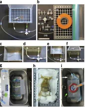
2.2 Building a PARS chamber
reagents may be collected from the catch-basin and recirculated back into a subject's vasculature; Luer-to-tubing couplers; and a Ziploc bag to contain the entire PARS chamber setup.
forewarning, SDS and salt precipitate will begin to accumulate within these narrow lines over time. It is important to flush the lines (e.g., with ddH2O) between subjects, and to replace occluded lines with new Tygon tubing (e.g., after every few subjects).
During hydrogel polymerization, the chamber must be enclosed inside a Ziploc freezer bag. To do this, disconnect the outer Tygon tubing that connects to the barbed connectors of the pipette tip box, and puncture three holes into the Ziploc bag to accommodate the 1/8 × 1/8-inch barbed connectors. Reconnect the Tygon tubing to their original 1/8 × 1/8-inch barbed connector. To connect a vacuum line to this bagged PARS box for withdrawing oxygen, tape a female Luer tee onto the lid of the pipette box and puncture one hole through the Ziploc. Finally, make the Ziploc airtight by placing clay around the punctured regions in the Ziploc.
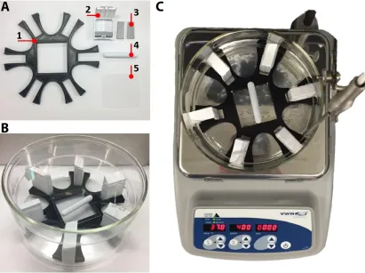
As a final note, a 1,000-μl tip box has a volume of ~750 ml. Thus, during hydrogel polymerization and during clearing, 200–300 ml of solution may be placed in the pipette box for recirculation without risk of the pipette box overflowing or the solution splashing out during its transport. Similarly, to conserve reagents during PARS clearing and immunostaining of smaller samples, a 200-μl tip box may be used to construct the PARS chamber; only 100 ml of reagent is necessary to fill such a chamber about one-third full (Figure 2.1).
2.3 Standardized Procedure for PARS
(pH 7.5), by clearing the buffer daily until the recirculated fluid is no longer yellowish, after which the SDS solution can be refreshed less frequently (every 48–72 h).
Check on the clearing progress daily. Add additional SDS buffer to the PARS chamber if necessary, as depending on how well the Ziploc bag is sealed around the perfusion tubing, some buffer may evaporate over time.
The sample can be continuously perfused for up to 2 weeks until all desired organs have cleared, even if some organs appear clear within the first 24–48 h. Alternatively, if all but one or two organs appear sufficiently transparent after a few days, one may proceed directly to Step 7C(iv) to flush SDS from tissue, and then excise all organs. The one or two semiopaque excised organs are transferred into 8% (wt/vol) SDS to finish clearing via PACT, whereas the organs that cleared more rapidly are immediately promoted to passive immunostaining (optional) and mounting without further delay.
2.4 Main Figures
[image:21.612.152.496.136.571.2]used to catheterize the heart. (i) The chamber is placed into a 37 °C water bath. A female Luer tee, which is taped onto the lid of the pipette tip box, is punctured through the Ziploc bag, and this joint is sealed with clay to ensure an airtight seal. Finally, to accelerate polymerization, a vacuum line is connected to the female Luer tee to remove oxygen (orange arrow), and a nitrogen gas line (white arrow) is connected to the 1/8-inch barbed connector to deliver a steady flow of nitrogen into the bagged system. The solute is continually circulated through the animal from the outflow line (blue arrow, which also indicates the direction of flow through blue-taped tubing) and inflow line (green arrow, which also indicates the direction of flow through green-taped tubing).
C h a p t e r 3
Bone CLARITY: clearing, imaging, and computational analysis of
osteoprogenitors within intact bone marrow
[2] Greembaum, A. et al. “Bone CLARITY: Clearing, imaging, and computational analysis of osteoprogenitors within intact bone marrow”. In: Science Translational Medicine 387.9 (2017). URL: http://doi.org/10.1126/scitranslmed.aah6518.
3.1 Summary
3.2 Introduction
The mammalian skeletal system consists of numerous bones of varying shapes and sizes that provide support to the body and protect internal organs from external physical stress21,22. Different bone types harbor specialized physiological processes that are key for proper development and survival of the organism, such as replenishment of hematopoietic cells, growth, and remodeling of the bone during healthy and diseased states23,24 25,26. Traditionally, these processes have been investigated through methods that provide zero- or two-dimensional information, such as fluorescence activated cell sorting (FACS) or analysis of histological sections. Quantitative 3D data of geometric features such as volume and number of cells, can be obtained from histological sections with unbiased stereological methods. Although statistically robust, such methods are labor-intensive and provide no visualization of the 3D structures. The need for methods that provide 3D information to study the bone has long been recognized. While methods such as serial sectioning and milling are valuable tools for understanding the structure of bone at the tissue level, these are destructive techniques that do not provide information at the cellular level and cannot be easily combined with other methods such as immunohistochemistry to characterize cellular processes27,28.
solvent-based clearing methods have achieved an imaging depth of approximately 200 µm using two-photon microscopy36. Murray’s clearing method was recently modified to clear bisected long bones and achieved an imaging depth of approximately 600 µm with confocal microscopy39. Despite these advances, manipulation and subsampling of the bone is required for deep imaging, thus disrupting the intact bone architecture. A key limitation of Murray’s clearing method and its variants is that they quench endogenous fluorescence, minimizing their application with transgenic fluorescent reporter lines, which are used to highlight key cell populations within the bone and marrow. Consequently, there is a need for a clearing method that maintains the intact bone structure, preserves endogenous fluorescence, and allows deeper imaging within intact bone without manipulation for sub-sampling.
3.3 Results
Bone CLARITY renders intact bones transparent while preserving endogenous fluorescence
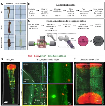
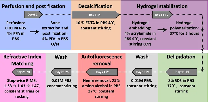
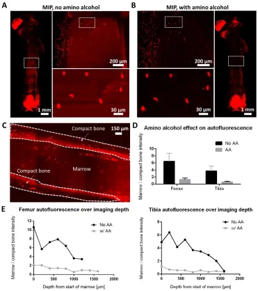
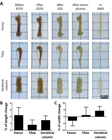
We developed and applied a bone clearing method to render the tibia, femur, and vertebral column of mice transparent for light-microscopy investigation (Fig. 1A). The key steps of the sample preparation including tissue clearing and autofluorescence removal are outlined in Fig. 1B and fig. S1. The bone is decalcified to increase light and molecular penetration through the tissue while leaving a framework of bone matrix with similar structural characteristics to dense fibrous connective tissue. DeCAL CLARITY employs an acrylamide hydrogel to support the tissue structure and minimize protein loss prior to the delipidation step. The detergent sodium dodecyl sulfate (SDS) is used to remove lipids in order to minimize their light scattering effects. We observed high autofluorescence in the bone marrow, one of the primary sites of heme synthesis. As heme is strongly autofluorescent, in the final step of the process we used the amino alcohol N,N,N',N'-tetrakis(2-hydroxypropyl)ethylenediamine40,41 to remove heme, which minimized marrow autofluorescence by approximately 3-fold (fig. S2). All of the above clearing stages were conducted on a temperature controlled stir plate that provides continuous convective flow (fig. S3, auxiliary design file). This accelerates and improves the clearing process for entire organs compared with passive clearing33. The samples did not change size during the clearing process (fig S4).
illuminated by only one of the two light-sheet paths, whichever provides the better contrast. We use only one illumination path per depth scan because there is always one illumination direction that scatters less light and thus provides superior image quality. To minimize RI mismatch between the objective lens and the bones, the samples are directly immersed in the immersion chamber without the use of a quartz cuvette to hold the sample. If RI variations still persist, the position of the detection objective is changed for each tile and specific depth along the Z-scan to mitigate any resulting out-of-focus aberrations. The LSFM captures images at a frame rate of 22 frames per second (16-bit depth) and produces 0.176 GB of imaging data per second. Large datasets are thus acquired for each imaged bone (50–500 GB). In order to manage these large datasets, we designed a computational pipeline that includes image stitching, automatic detection of individual cells, and volume of interest (VOI) rendering for analysis (Fig. 1C).
To validate the protocol, we applied our clearing and imaging method to locate progenitor cells in the long bones and vertebrae of transgenic reporter mice. A Sox9CreER transgenic mouse line was used in which, upon tamoxifen injection, multipotent osteoblast and chondrocyte progenitor cells express tdTomato21,46. We visualized the endogenous fluorescence of Sox9+ cells using Bone CLARITY (Fig. 1D and E). Quantification of the imaging depth in different regions of the tibia, femur, and vertebral body showed that we were able to image through the diaphysis of the femur (movie S1) and tibia (movie S2) and the entire vertebral body (movie S3). Furthermore, we were able to reliably detect Sox9+ cells up to approximately 1.5 mm deep into the bones (fig. S6). Collectively, deCAL CLARITY coupled with LSFM and the data-processing pipeline is an effective clearing, imaging, and data processing protocol to investigate intact mouse bones.
Semi-automated computational pipeline quantifies Sox9+ cells in mouse tibia
and femur
CLARITY allows for detection and quantification of individual Sox9+ cells in 3D (Fig. 2A), some of which appear associated with small vessels. Owing to the large VOI (Fig 2A, gray surface), we created a semi-automated cell-detection algorithm (Fig. 2B and fig. S7). The algorithm divides the 2D images that make up the Z-stack (or depth scan) into N small overlapping regions, and then adaptively thresholds the 2D images into binary images on the basis of the local mean and standard deviation of fluorescence. The resulting binary 2D images are further subject to morphological operations to eliminate noise and discontinuity within a cell. All of the 2D binary images are then combined into a 3D matrix. From the 3D matrix, only volumes that fit the properties of a Sox9+ cell are maintained, thus avoiding erroneous counting of large blood vessels or small autofluorescence artifacts. All cells outside the user-defined VOI (Fig. 2A) are discarded. The cell candidate centroid locations are then imported to 3D visualization software for quality control. During the quality control stage, the annotator reviews the entire 3D volume and corrects the automatic results by marking false negative cells and omitting false positive cells. Therefore, at the end of the quality control stage, the cell counts are equivalent to cell counts that are performed manually. According to our experiments, a fully automatic pipeline only achieves on average 52% sensitivity and 36% precision. It should be noted that removing false positives is a faster operation in the 3D visualization software than adding false negatives, therefore the value of sensitivity outweighs the need for precision.
diaphysis reside adjacent to the endocortical surface, with mean distances from the periosteal surface of approximately 136.9 µm and 143.6 µm for the tibia and femur, respectively (Fig. 2E). This result supports similar findings in48 and validates deCAL CLARITY as a reliable method to resolve and quantify individual cells in intact bone and marrow spaces. It should be noted that Bone CLARITY is not limited to visualize cell populations in transgenic animals only and that antibody staining is also feasible (fig. S10). However, for maximum penetration of the antibody into the bone, it is recommended to bisect the bone prior to the clearing process.
Bone clearing can complement section-based stereology
Design-based stereology is the gold standard method to quantify total cell numbers and densities in organs while preserving spatial information49. Stereology relies on statistical sampling methods. Systematic uniform random sampling (SURS) is a frequently used sampling method that efficiently reduces the variance of the estimate compared with random sampling. SURS obtains histological sections from an organ to reduce the amount of tissue for analysis. SURS samples at regular uniform intervals with the first sample collected at a position random within the first interval50,51. The number of cells in a tissue volume is a zero-dimensional geometric feature, and to avoid bias based on the cell size or shape, a probe based on two thin physical sections or optical planes separated by a known distance (disector), is used to accomplish quantification5253. Cells are typically counted in a known fraction of the organ, which allows for an estimation of the total number of cells in the entire organ54. The spatial distribution of cells can also be obtained using second-order stereological methods55.
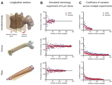
representative selection of N random uniformly spaced sections for a simulated SURS experiment in the femur, tibia, and vertebral body. Fig. 3B shows the estimates for the cell count of an entire VOI based on N sampled slices, and Fig. 3C illustrates the coefficient of variation of simulated stereology experiments that were conducted with N slices. To estimate the coefficient of variation for each N representative slices, 5 simulated stereology experiments were conducted. In these simulations, as expected, variance decreased rapidly with increasing number of slices for femur, tibia, and vertebrae. Precision of the stereological estimate would likely be improved with proportionator sampling, a form of non-uniform sampling better suited to rare structures56. Therefore, the 3D counting method offers several advantages for quantifying rare cellular populations: the ability to detect subtle changes that might be overlooked because of sampling variance, elimination of the need for sectioning, and 3D visualization.
Sclerostin antibody increases the number of Sox9+ cells in the vertebral column
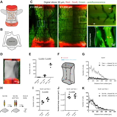
quantification of vertebral Sox9-tdTomato cells after tamoxifen administration versus the two control groups, Sox9CreER mice without tamoxifen administration and wild-type mice, can be seen in Fig. 4E. Again, we observed that the Sox9CreER transgenic animals without tamoxifen administration display mild leakage of tdTomato expression (Fig. 4E and fig. S9). Overall, similar to the cell distribution results presented for the tibia and femur, the Sox9+ cells were primarily located adjacent to the endocortical surface (Fig. 4, F and G), with a mean distance of 138.8 µm and 137.6 µm for the tamoxifen-negative (Tam.-) and tamoxifen-positive (Tam.+) groups, respectively.
surface to contribute to the increase in osteoblast number. The distribution of cells as a function of distance from the surface can be seen in Fig. 4K, with mean distances of approximately 99.9 µm and 137.8 µm for the vehicle and treated groups, respectively. 3.4 Discussion
In the bone remodeling process, bone health is maintained through continuous cycles of bone resorption by osteoclasts and bone formation by osteoblasts. Imbalances in these physiological processes can lead to various bone diseases such as osteoporosis, which affect millions of people in the United States alone57,60. In order to gain better insight into potentially effective treatments for osteoporosis, it is imperative to study the physiological processes that occur in healthy and diseased bone and understand the molecular and cellular mechanisms within the 3D microenvironment. We demonstrate that the Bone CLARITY technique renders the tibias, femurs, and vertebral bodies of mice optically transparent while preserving bone morphology and an endogenous fluorescent reporter signal. In addition to matching the RI of the tissue, Bone CLARITY also removes minerals and lipids, thus enabling us to reconstruct a whole vertebral body as well as the entire diaphysis from the tibia and femur.
deCal CLARITY do introduce a compromise in processing time (28 days). Utilizing faster decalcification agents, such as formic acid, might shorten the current decalcification time of 14 days albeit the fluorescent proteins generated by the reporter genes used in this study might lose their fluorescence under acidic conditions42,62. Delipidation is also a lengthy stage in Bone CLARITY but necessary to reduce scattering from lipids present not only in the mineralized bone tissue, but highly abundant within the bone marrow. Consequently, delipidation ensures high-quality optical access deep in the bone. Although the use of customized microscopy and software might not be easy to implement in a non-technical setting, commercial LSFM systems with a streamlined user interface and associated software are rapidly evolving to support the types of application described here. For data processing, we found that fully automated cell-detection algorithms were difficult to apply within cleared tissue. SNR variations arising from non-uniform illumination and fluorescence detection within the bone resulted in unsatisfactory precision, necessitating manual quality control. The simple automated tools that we developed are fast and adaptive and in general are able to save annotator time while improving precision and reducing error; however, more work is required to achieve a reliable, fully automated algorithm for cell counting. In general, data handling, visualization, and analysis would benefit from individual developers sharing their code in an open-source environment, which would allow the scientific and medical community to efficiently customize software relevant for the application at hand.
complicated structural elements cannot be done automatically. Therefore, subsampling is advantageous for manual quantification within a reasonable timeframe. Finally, to further demonstrate the utility of our clearing method, we treated a cohort of adult reporter mice with a sclerostin antibody, a bone-forming agent, for 9 days. Previous stereological studies in rats treated with Scl-Ab for 8 days revealed a dramatic increase in total osteoblast number in the vertebrae coincident with increased bone formation, but no significant effect on bone progenitor numbers58. We found that, after 9 days of treatment in mice, the total number of osteoblast progenitor cells increased by 36% compared with the control group. This result was not surprising based on the literature58, but it has been challenging to demonstrate using stereological methods given the rarity of osteoprogenitor cells, particularly in the vertebrae. This underscores the greater sensitivity of our clearing, imaging, and data-processing protocol for quantifying rare cell populations as well as using lineage tracing to mark progenitors, as opposed to immunophenotyping in tissue sections. Overall, continued developments in tissue clearing 6,32,34, imaging, and data analysis can facilitate translational research that will provide insight into the efficacy and safety of new bone-modulating drugs by profiling their effects on progenitor cell populations.
3.5 Main figures
Fig. 1. Bone CLARITY renders intact bones transparent while preserving endogenous fluorescence. (A) Micrographs of mouse tibia, femur, and vertebral column before and after CLARITY. Bones were rendered transparent using deCAL CLARITY. (B) Block diagram outlining of the key steps of Bone CLARITY sample preparation. The procedure includes: demineralization, hydrogel stabilization, lipid removal via constant flow, and autofluorescence removal. (C) A schematic diagram of the imaging and computational
B A
C
Sample preparation
Image acquisition and processing pipeline
Imaging using light-sheet microscopy 3D surface creation Manual quality control of cell counting
Red - Sox9, Green - autofluorescence
T ib ia F e m u r V e rt e b ra l c o lu m n Pre-clearing DeCAL-CLARITY 6 mm
Greenbaum, Chan, et al., 2017 FIGURE 1
D Tibia, MIP
Z = 1 1 0 0 µ m Z = 3 0 0 µ m
Tibia, digital slices 30 µm
Marrow Compact bone C o m p a c t b o n e Marrow Compact bone C o m p a c t b o n e
Vertebral body, MIP
E
1 mm
100 µm
200 µm 20 µm
(Day 0) (Day 14) (Day 15) (Day 21) (Day 28)
Perfusion and fixation Mineral removal with EDTA Flow mediated clearing Auto- fluorescence quenching Bone cleared and ready for imaging Hydrogel stabilization (Day 1) Automatic cell detection and 3D visualization Statistical analysis 3D visualization Image processing platform
[image:36.612.121.526.131.538.2]Fig. 2. Bone CLARITY enables quantification of fluorescently labeled Sox9+ cells in the
mouse tibia and femur. (A) Femur MIP fluorescent image and magnified images showing single Sox9+ cells in the vicinity of the third trochanter (red = Sox9 and green = autofluorescence). The gray surface surrounding the femur represents an overlay of the volume of interest (VOI); only the cells that reside within the VOI are quantified. The purple, blue and yellow boxed regions in the MIP represent progressive magnification.(B) Block diagram of the semi-automated cell detection pipeline where cell candidates are identified via adaptive thresholding and their volume calculated. A predetermined selection criterion
A Femur, MIP, Red - Sox9, Green - autofluorescence
B
Convert to a 3D binary map Stitched images
Reject 3D volumes that are too large or small to be cells and locate
centroids
Export centroids of detected cells to 3D visualization software for quality
control Divide the image
into N overlapping regions
Adaptively threshold each tile for finding
cell candidates For every 2D image in the image stack
Cell detection pipeline
Rejected = volume is too large or out of user defined surface
D
Distance from surface
Sox9 cell B o n e s u rf a c e E 1 mm
100 µm 50 µm
1 mm
Distance from surface [µm]
N u m b er o f ce lls Femur (n=3) Tibia (n=3) C N u m b e r o f c e lls Tibia N u m b e r o f c e lls Femur
P = 0.0120
0 200 400 600 800 0 50 100 150 200 0 400 800 1200
1600 Sox9+, Tam.+
Greenbaum, Chan, et al., 2017
WT
n =
3
Tam
.-n =
3
Tam
.+
n =
3 0 200 400 600 800
1000 P = 0.0002P = 0.0008 P = 0.0020
WT
n =
3
Tam
.-n =
3
Tam
.+
n =
[image:38.612.123.524.102.504.2]Fig. 3. Using intact tissue clearing methods reduces cell estimate variability compared with traditional tissue sectioning methods. (A) Schematic diagram showing the sample selection procedure for systematic uniform random sampling (SURS) of the mouse femur, tibia, and vertebral body. N uniformly spaced 2D sections are selected, offset by a random starting distance. The red single arrow indicates the random starting point, while the double arrow indicates the distance between the 2D sections. (B) Sox9+ cell number estimation as a function of the number of sampled sections in a representative simulated stereology experiment using both SURS (red dots) and simple random sampling (blue dots). To simulate a stereology experiment, the cell density in the sampled sections is used to interpolate the cell number in the entire VOI. The black dashed line represents the ground truth, cell number based on the entire volume. (C) The coefficient of variation of five simulated stereology cell number estimates as a function of the number of sampled slices using SURS (red dots) and simple random sampling (blue dots).
Longitudinal sections B Simulated stereology Coefficient of variation A
Random starting point
Greenbaum, Chan, et al., 2017
experiment of 6 µm slices C across multiple experiments
V e rt e b ra l b o d y 600
Number of slices sampled
E s ti m a te d n u m b e r o f c e lls
0 50 100 150 200
0 200 400
1.2
Number of slices sampled
C o e ff ic ie n t o f v a ri a ti o n
0 50 100 150 200
0.0 0.4 0.8 F e m u r
Number of slices sampled
E s ti m a te d n u m b e r o f c e lls
0 50 100 150 200
0 500 1000 1500 Random SURS T ib ia
Number of slices sampled
E s ti m a te d n u m b e r o f c e lls
0 50 100 150 200
0 500 1000 1500
Number of slices sampled
C o e ff ic ie n t o f v a ri a ti o n
0 50 100 150 200
0.0 0.4 0.8 1.2
Number of slices sampled
C o e ff ic ie n t o f v a ri a ti o n
0 50 100 150 200
[image:40.612.128.517.103.397.2]Fig. 4. Bone CLARITY enables quantification of the effect of sclerostin antibody on the number of fluorescently labeled Sox9 cells in the mouse vertebra. (A) Schematic depicting the lateral view of a mouse vertebra. The intervertebral disk is labeled in red; chondrocytes proliferate there after differentiation from tdTomato-Sox9+ cells (chased for 7 days). The marrow is represented in light orange. (B) Transverse view of an L4 vertebra. The cell counts are isolated to the vertebral body, and the dashed lines approximate the locations of the sections shown in C. (C) Digital sections (30 m thick) at different depths along the vertebral body (Z = 200 m and 650 m), red = Sox9 and green = autofluorescence. The
Spinal cord
Vertebral body Late
ral p roc ess e s Spinous process Vertebral body Intervertebral disc A B
C Digital slices 30 µm, Red - Sox9, Green - autofluorescence
D E F G
Scl-Ab Scl-Ab
and Tam. End of study
4 days 5 days
H
Distance from surface
Sox9 cell
Z = 200 µm Z = 650 µm
200 µm 50 µm
200 µm N u m b e r o f c e lls K I N u m b e r o f c e lls
Scl-A
b-n=5 Scl-A
b+ n=4 N u m b e r o f c e lls
Distance from surface [µm] Distance from surface [µm]
0 200 400 600 800 1000 Wild type
n=3 Sox+; Tam
.-n=3Sox+; Tam .+ n=4 N u m b e r o f c e lls J V er te b ra l b o d y v o lu m n [ µ m 3]
1 109
2 109
3 109
4 10x 9
x
x
x Sox9+ and Tam.+
Scl-A
b-n=5 Scl-A b+
n=4
Sox9+ and Tam.+ Sox9+ and Tam.+
0 100 200 300 400 500 600 0 20 40 60 80 100
Tam. +, chased 7d, n=4 Tam. - , chased 7d, n=3 Sox9+
Scl-Ab-, chased 5d, n=5 Scl-Ab+, chased 5d, n=4
0 200 400 600 800 1000
Greenbaum, Chan, et al., 2017
C o m p ac t b o n e
P = 0.0311P = 0.0002
P = 0.0183 P = 0.3403
L ate ra l p roc es se s
[image:41.612.120.525.104.509.2]3.6 Supplementary Figures
Fig. S1. Bone CLARITY clearing process. (A) As a first step (blue) in Bone CLARITY
method transcardial perfusion is performed with 0.01M PBS, pH 7.4, and 4%
paraformaldehyde (PFA) in PBS, pH 7.4. Hard tissue is then extracted and post-fixed with
4% PFA in PBS, pH 7.4 at 4°C for 16 hours. Hard tissue is then decalcified (orange). During
this step, daily-exchange of 10% EDTA in PBS, pH 8, at 4°C under constant stirring is
performed. Hydrogel stabilization to prevent protein loss is carried out (purple). The tissue
is incubated in a hydrogel composed of 4% acrylamide with 0.25% VA044 in PBS at 4°C
under constant stirring for 16 hours. Afterwards, the hydrogel is degased with nitrogen gas
and polymerized at 37°C. Delipidation is carried out with 8% SDS in PBS, pH 7.4 at 37°C
under constant stirring (green). A wash step with PBS is performed before heme removal
from the tissue (gray). Heme removal is performed with 25% amino alcohol in PBS, pH 9,
at 37°C under constant stirring (red). A second wash step is performed on the tissue (gray).
Finally, the tissue is refractive index matched to 1.47 through daily step-wise buffer exchange
Fig. S6. Signal quality metrics to quantify imaging depth of Bone CLARITY. (A) MIP of a cleared mouse femur with estimates of imaging depth limit at different anatomical regions. The arrows indicate the direction of analysis and the calculated imaging depth. (B) Examples of isolated Sox9+ cells at different imaging depths and in different bone regions. Sox9+ cells remain
distinguishable at the deepest parts of the metaphysis and diaphysis, but signal loss is evident in the deeper parts of the epiphysis. The same analysis was repeated for a cleared mouse tibia (C) and vertebra (D). (E) The peak signal-to-noise ratio (PSNR) of isolated Sox9+ cells. The dashed
3.7 Supplementary movie captions
Movie S1: Visualizing endogenous fluorescence throughout a cleared mouse femur. The movie shows a MIP image of an entire mouse femur at different angles and zoomed in view of the greater trochanter area. Digital sections with 30 µm thickness are shown at different bone depths at the greater trochanter. Sox9+ cells are labeled with red fluorescent protein (tdTomato), while tissue autofluorescence in green provides structural cues. (doi:10.22002/D1.234)1
Movie S2: Visualizing endogenous fluorescence throughout a cleared mouse tibia. MIP image of an entire mouse tibia rotated in different angles. Zoomed in digital sections (30 µm thick) of the tuberosity and the diaphysis are shown. The Sox9+ cells are labeled with tdTomato and tissue autofluorescence in green for structural orientation. When the red channel is turned off (Z = 2016 µm) some cellular processes can be seen. (doi:
10.22002/D1.235) 1
Movie S3: Visualizing endogenous fluorescence throughout a cleared mouse vertebral body. The movie shows an L4 vertebra body of a mouse. The intervertebral disks labeled in red can be seen in the vertical edge of the image. Longitudinal sections (30 µm thick) of the vertebra body at different depths can also be seen where the red channel shows Sox9+ cells and the green channel shows tissue autofluorescence. (doi: 10.22002/D1.236) 1
3.8 Materials and methods
Study design: The objective of this study was to enable the visualization and quantification of cell population in an intact bone tissue by developing and integrating tissue clearing, fluorescence microscopy, and a computation pipeline. Experimental and control animal cohorts were chosen based on preliminary data that suggested a large effect size. All transgenic animals used in this study are as described in the animals section. All wild-type animals used in this study were C57BL/6. To characterize the density of sox9+ cells and distribution within the femur, tibia and vertebral column, male transgenic animals of 6-7 weeks of age received a 2 mg tamoxifen IP on day 1 of the experiment to enable expression of a native fluorescent gene for 7 days before culling. For the study of the effects of sclerostin-antibody on total number of osteoprogenitor cells, a cohort of 7 weeks old male transgenic animals were treated with a sclerostin antibody at 100 mg/kg IP on day 1, and again 4 days later at 100 mg/kg IP with tamoxifen induction at 2 mg IP before culling on day 9 of the study. The sclerostin antibody was provided by Amgen. During cell counting all manual quantification is performed in a blind manner to eliminate observer bias. Animals were randomly assigned to groups for experiments. Raw data values for cell counts are reported in an auxiliary supplementary file.
Massachusetts, pH 7.8) via HYDROPAC. Animals were maintained on a 12:12 hour light:dark cycle in rooms at 64-79 F with 30-70% humidity under pathogen-free conditions.
Bone deCAL CLARITY protocol: The clearing process is summarized in fig. S1. After euthanization, mice were perfused transcardially with 0.01M PBS (Sigma, #P3813) followed by 4% paraformaldehyde (PFA) (VWR, #100496-496) and the femurs, tibias and L3-5 vertebral columns were extracted. The bones were post-fixed overnight in 4% PFA. To enhance clearing of hard-tissue, the demineralization phase was extended to 2 weeks with 10 % EDTA (Lonza, # 51234) in 0.01M PBS, pH 8. During the demineralization phase, samples were kept under constant stirring in histology cassettes (Electron Microscopy Sciences, #70077-W) at 4°C with fresh EDTA buffer exchanges daily. Next, the decalcified bones were embedded in a hydrogel matrix (A4P0) which consist of 4% acrylamide (Bio-Rad, #1610140), 0% paraformaldehyde, and 0.25% thermo-initiator A4P0 (Wako Chemicals, VA-044) in 0.01M PBS overnight at 4°C. The samples were degassed through nitrogen gas exchange for 5 minutes and polymerized at 37°C for 3 hours. After structural reinforcement with the A4P0 hydrogel, delipidation was carried out with 8% SDS in 0.01M PBS, pH 7.4, for 4 or 5 days (vertebral body and long bones respectively) at 37°C under constant stirring (fig. S3). The samples were then washed for 48 hours in 0.01M PBS with 3 buffer replacements. The amino alcohol N,N,N',N'-tetrakis(2-hydroxypropyl)ethylenediamine (Sigma, #122262-1L) was added at 25% W/V in 0.01M PBS, pH 9, for 2 days at 37 °C under constant stirring for the purpose of decolorization of the tissue through heme group removal. Lastly, the bones were washed with 0.01M PBS for 24 hours and subsequently immersed in refractive index matching solution (RIMS). The bones were gradually immersed in RIMS (15) with a refractive index of 1.47 through daily step-wise RIMS exchange starting with RIMS 1.38, RIMS 1.43 and finally RIMS 1.47.
collar on the objective lens (10× CLARITY Objective lens with numerical aperture of 0.6, Olympus XLPLN10XSVMP) was set accordingly. To image the entire bone, multiple tiles with 10% overlap were acquired. Typically, the femur, tibia and vertebral body required 13×5, 11×5 and 3×2 tiles respectively (vertical × horizontal). In a calibration stage that took place prior to the scan, the following parameters were defined for each tile: (i) Light-sheet illumination direction; the LSFM has two light-Light-sheets that illuminate the sample from opposite directions. Selecting the preferable illumination direction dramatically reduced scattering. (ii) The start and end point of the Z-stack; this step was done in order to minimize the number of acquired images in an already big data set (50-500 GB). (iii) The focus points of the detection objective along the scan were defined to mitigate RI variations along the scan that created out-of-focus aberrations. Once the calibration stage was completed, the bone was imaged with a frame rate of 22 frames per second, and bit depth of 16 bits. The acquired data set size depends on the sampled voxel size. For a voxel size of 0.585×0.585×2 µm3 the tibia and femur produced ~ 250 GB of data per color channel, while the vertebral body produced ~ 30 GB of data per color. Generally, the datasets are down-sampled after acquisition for processing; the typical voxel sizes are 1.17×1.17×2 µm3 and 2.34×2.34×2 µm3 for the vertebra column and long bones respectively.
All experimental and control groups were imaged with the same laser power. For images that were acquired deep in the bone and when the SNR changed within the distance from the bone boundary, the contrast and gamma were adjusted in the displayed images. The gamma adjustment was done to visualize cells that exhibit both low and high intensity within the same field-of-view. Images from the vertebra (Sox9+ and Tam+ group) are representative of 13 vertebrae from 13 mice. Images from the tibia and femur (Sox9+ and Tam+ group) are representative of 5 tibias and 5 femurs from 5 mice.
3.9 Supplementary methods
Computational pipeline: LSFM generates multidimensional datasets on the order of hundreds of gigabytes, for example 500 GB for tibia with 2 color channels, motivating a necessity for high-throughput automated computational tools to do data processing, management, and visualization. Thus, we established a computational pipeline optimized for large datasets that interfaces between 3D visualization and analysis software (Imaris, Bitplane) and a programming framework (Matlab, Mathworks) although alternatives can also be used (e.g. Amira, Python).
Tile stitching was done with TeraStitcher. The acquired tiles (.tiff format) were saved according to the TeraStitcher two-level hierarchy and file naming convention. The resulting stitched tiles were saved as large individual.tiff format file per Z section. To accelerate processing and manipulation of 3D images in Imaris, the lateral resolution was down-sampled by a factor of 2 and 4 for vertebrae and long bones, respectively. These image stacks were then converted into a single large multiresolution 3D Imaris image. The 3D image is then used to construct the VOI, performing quality control for the automatic cell detector, and obtaining relevant statistics about the position of the cells within the VOI.
Using Imaris surface tools, a VOI was constructed around the bone surface, while excluding connective tissue. The VOI was used to count cells and evaluate morphology (fig. S7). For the femur and tibia, the VOI was defined around known anatomical regions: the third trochanter and tibial crest, respectively. The surface for the vertebral body aimed to surround the inner marrow of interest and exclude surrounding compact bone and chondrocyte-dense endplates.
binary format and morphological operations are conducted to improve connectivity and discard noise. A 3D binary matrix is then constructed from the 2D binary images and connected voxels are grouped into 3D blobs. Blobs that showed one of the following criteria were removed: (i) blobs with volume outside of a 523-33,500 µm3 range, (ii) blob with spatial position outside of the VOI and (iii) blobs that show strong signal in the autofluorescence channel. The centroids of the remaining blobs are imported into Imaris to perform manual adjustments. The goal of the automatic detection is to facilitate manual detection by saving time and reducing the chance of error from long annotation sessions.
Using Imaris’ clipping plane tool, the 3D image is divided into thick slices (~ 100 µm) to allow for manual adjustments of the automatically detected cells. Viewing cells in these thick sections allows for visualization of 3D features that help to accurately identify cells. When counting the cells, 2 color channels were used to disambiguate between autofluorescence (green) and the true Sox9+ signal (red). If the Sox9+ cell under question is present with strong intensity in the autofluorescence channel, then it was not included in the quantification.
Following manual cell count adjustments, Imaris was used to generate distance to surface and cell count statistics. The surface was imported into Imaris’ cell object with the marked Sox9+ spots as its vesicles. Automatically generated statistics were imported to Matlab for further processing and plotting.
Sample mounting for light-sheet microscope: To mount the sample for LSFM, one end of a 4 cm long plastic capillary was flattened using a plier, and a small amount of All Purpose Krazy Glue (KG585) was applied on this end. The flattened end was later placed on the edge of the cleared condyles (femur) and L3 (vertebral column) bone while moderate pressure was applied. Four minutes later, the capillary bonded with the bone and the sample was placed back into RIMS. Before imaging, the plastic capillary was fitted to a glass capillary, which can be attached to the sample stage of the LSFM (fig. S5).
datasets. To start, the coordinates of each cell center were imported to MATLAB as a list, and the VOI was imported to MATLAB as a binary mask. From the binary mask, the volume of each 2D section was calculated by accumulating the number of pixels in the 2D section and multiplying it by the voxel size. Then, a simple random sampling stereology experiment was simulated by stochastically selecting N digital sections (6 μm thick) from the entire VOI. Only cells whose centroids were within the volume of the selected digital sections were counted, this guarantees that each cell will be counted only once and cell will not be overrepresented. To calculate the cell density, the total number of counted cells in the selected digital sections was divided by their accumulated volume. From sampled cell density and the known volume of the entire bone, the total number of cells in the bone was estimated. In order to calculate the coefficient of variation, each experiment was repeated 5 times and the standard deviation of the experiments was divided by the total cell number of the volume. To reflect modern stereology sampling techniques, we also simulated systematic uniform random sampling (SURS) stereology experiments. As compared to simple random sampling, SURS has a stricter subset of possible samplings. Rather than looking at any random subset of slices, SURS requires sampling the tissue with a fixed interval, while the first starting slice is randomly selected (Fig. 3A). In order to compare SURS with simple random sampling, each SURS experiment consisted of a specific number of digital slices. Since a specific number of digital slices can be attained by a variety of sample intervals, the minimum interval that would yield the desired number of slices was selected. Once the digital sections were selected for SURS, the cell density was calculated in the same manner as simple random sampling. To calculate the coefficient of variation, each SURS experiment was repeated for 5 random starting positions. Figure 3C shows only numbers of slices that yielded at least 5 possible starting positions.
both sufficient compact bone and marrow for analysis. Then, for 7-9 depths along the imaging dimension, two areas (~ 1000 µm2) were extracted. The first area exclusively contained compact bone, while the other exclusively contained marrow. The mean intensities of the two areas (marrow and compact bone) were then calculated. The mean intensity ratio (marrow versus compact bone) was used to quantify the amino alcohol effect on quenching auto-fluorescence in the marrow, since amino alcohol operates on heme, which is found only in the marrow. To verify that amino alcohol did not quench endogenous fluorescence, we compared the same region of the bone before and after amino alcohol treatment (fig. S2).
Quantifying imaging depth at different anatomical regions of the bone (related to fig.
S6): Bone tissue is difficult to clear and image in 3D, particularly in deeper regions where the SNR is low. Additionally, bones are highly heterogeneous and different regions have significantly different biological makeup that affects imaging SNR. In order to characterize the imaging depth capabilities of LSFM in bone tissue cleared by Bone CLARITY, we quantitatively assessed cell detection in several anatomically distinct regions using a Peak SNR (PSNR) metric (equation 1).
𝑃𝑆𝑁𝑅 = 20 × log10 𝑀𝐴𝑋−𝜇
𝜎 (1)
with high concentration of chondrocytes, no isolated cells could be found, thus creating large gaps along the imaging depth in fig. S6E.
3.10 Additional information
Acknowledgements: We thank Antti Lignell and Long Cai for technical help in building the LSFM and the Amgen Scientific Team (Frank Asuncion, David Hill, Mike Ominsky and Efrain Pacheco). Alon Greenbaum is a Good Ventures Fellow of the Life Sciences Research Foundation.
Funding: NIH Director's New Innovator IDP20D017782 and PECASE; Heritage Medical Foundation; Curci Foundation; Amgen-CBEA; Pew Charitable Trust; Kimmel Foundation; Caltech-COH.
Author contributions: H.J.McB. and V.G. conceived the project; A.G. and K.C. performed all experiments, data acquisition and analysis; T.D. and D.B. contributed computational tools and data analysis with input from R.B.; D.H.B. and H.M.K. contributed samples for clearing. A.G., K.C., T.D., D.B., and V.G. generated the figures and wrote the manuscript with input from all authors. V.G. supervised all aspects of the work.
Competing interests: V.G., K.C. and A.G. are inventors on patent application CIT-7683-P filled by California Institute of Technology that covers methods and devices for soft and osseous tissue clearing and fluorescent imaging. H.J.McB and R.B. are employees and shareholders of Amgen, Inc.
C h a p t e r 4
Engineered adeno-associated viruses for efficient and noninvasive gene
delivery throughout the central and peripheral nervous systems
[1] Chan, K.Y.C et al. “Engineered adeno-associated viruses for efficient and noninvasive gene delivery throughout the central and peripheral nervous systems”. In press.
4.1 Summary
4.2 Introduction
Adeno-associated viruses (AAVs)14 have been extensively used as vehicles for gene transfer to the nervous system enabling gene expression and knockdown, gene editing64,65, circuit modulation1,66, in vivo imaging67,68, disease model development69, and the evaluation of therapeutic candidates for the treatment of neurological diseases70. AAVs are well suited for these applications because they provide safe, long-term expression in the nervous system71,72. Most of these applications rely on local AAV injections into the adult brain to bypass the blood-brain barrier (BBB) and to temporally and spatially restrict transgene expression.
Targeted AAV injections have also been used for gene delivery to peripheral neurons to test strategies for treating chronic pain73-75 and for tracing, monitoring, and modulating specific subpopulations of vagal neurons76,77. Many peripheral neuron populations, however, are difficult to access surgically (e.g., dorsal root ganglia (DRG), nodose ganglia, sympathetic chain ganglia, and cardiac ganglia) or are widely distributed (e.g., the enteric nervous system), thereby limiting methods for genetic manipulation of these targets. Likewise, in the CNS, single localized injections may be insufficient to study circuits in larger species78 or to test gene therapies for diseases that involve the entire nervous system or widely distributed cell populations (e.g., Parkinson’s, Huntington’s, amyotrophic lateral sclerosis, Alzheimer’s, spinal muscular atrophy, Friedreich’s ataxia, and numerous lysosomal storage diseases)70.