Rapid Learning In Robotics pdf

(1)

(2)

Walter, Jörg

Rapid Learning in Robotics / by Jörg Walter, 1st ed. Göttingen: Cuvillier, 1996

Zugl.: Bielefeld, Univ., Diss. 1996 ISBN 3-89588-728-5

Copyright:

c

1997, 1996 for electronic publishing: Jörg Walter

Technische Fakultät, Universität Bielefeld, AG Neuroinformatik PBox 100131, 33615 Bielefeld, Germany

Email: [email protected]

Url: http://www.techfak.uni-bielefeld.de/walter/

c

1997 for hard copy publishing: Cuvillier Verlag

(3)

Jörg A. Walter

Rapid Learning in Robotics

Robotics deals with the control of actuators using various types of sensors and control schemes. The availability of precise sensorimotor mappings – able to transform between various involved motor, joint, sensor, and physical spaces – is a crucial issue. These mappings are often highly non-linear and sometimes hard to derive analytically. Consequently, there is a strong need for rapid learning algorithms which take into account that the acquisition of training data is often a costly operation.

The present book discusses many of the issues that are important to make learning approaches in robotics more feasible. Basis for the major part of the discussion is a new learning algorithm, the Parameterized Self-Organizing

Maps, that is derived from a model of neural self-organization. A key

(4)

Foreword

The rapid and apparently effortless adaptation of their movements to a broad spectrum of conditions distinguishes both humans and animals in an important way even from nowadays most sophisticated robots. Algo-rithms for rapid learning will, therefore, become an important prerequisite for future robots to achieve a more intelligent coordination of their move-ments that is closer to the impressive level of biological performance.

The present book discusses many of the issues that are important to make learning approaches in robotics more feasible. A new learning al-gorithm, the Parameterized Self-Organizing Maps, is derived from a model of neural self-organization. It has a number of benefits that make it par-ticularly suited for applications in the field of robotics. A key feature of the new method is the rapid construction of even highly non-linear

vari-able relations from rather modestly-sized training data sets by exploiting

topology information that is unused in the more traditional approaches. In addition, the author shows how this approach can be used in a mod-ular fashion, leading to a learning architecture for the acquisition of basic skills during an “investment learning” phase, and, subsequently, for their rapid combination to adapt to new situational contexts.

The author demonstrates the potential of these approaches with an im-pressive number of carefully chosen and thoroughly discussed examples, covering such central issues as learning of various kinematic transforms, dealing with constraints, object pose estimation, sensor fusion and camera calibration. It is a distinctive feature of the treatment that most of these examples are discussed and investigated in the context of their actual im-plementations on real robot hardware. This, together with the wide range of included topics, makes the book a valuable source for both the special-ist, but also the non-specialist reader with a more general interest in the fields of neural networks, machine learning and robotics.

(5)

iii

Acknowledgment

The presented work was carried out in the connectionist research group headed by Prof. Dr. Helge Ritter at the University of Bielefeld, Germany.

First of all, I'd like to thank Helge: for introducing me to the exciting field of learning in robotics, for his confidence when he asked me to build up the robotics lab, for many discussions which have given me impulses, and for his unlimited optimism which helped me to tackle a variety of research problems. His encouragement, advice, cooperation, and support have been very helpful to overcome small and larger hurdles.

In this context I want to mention and thank as well Prof. Dr. Gerhard Sagerer, Bielefeld, and Prof. Dr. Sommer, Kiel, for accompanying me with their advises during this time.

Thanks to Helge and Gerhard for refereeing this work.

Helge Ritter, Kostas Daniilidis, Ján Jokusch, Guido Menkhaus, Christof Dücker, Dirk Schwammkrug, and Martina Hasenjäger read all or parts of the manuscript and gave me valuable feedback. Many other colleagues and students have contributed to this work making it an exciting and suc-cessful time. They include Jörn Clausen, Andrea Drees, Gunther Heide-mannn, Hartmut Holzgraefe, Ján Jockusch, Stefan Jockusch, Nils Jung-claus, Peter Koch, Rudi Kaatz, Michael Krause, Enno Littmann, Rainer Orth, Marc Pomplun, Robert Rae, Stefan Rankers, Dirk Selle, Jochen Steil, Petra Udelhoven, Thomas Wengereck, and Patrick Ziemeck. Thanks to all of them.

(6)

(7)

List of Figures

2.1 The Puma robot manipulator . . . 10

2.2 The asymmetric multiprocessing “road map” . . . 11

2.3 The Puma force and position control scheme . . . 13

2.4 [a–b] The endeffector with “camera-in-hand” . . . 15

2.5 The kinematics of the TUM robot fingers . . . 16

2.6 The TUM hand hydraulic oil system . . . 17

2.7 The hand control scheme . . . 18

2.8 [a–d] The sandwich structure of the multi-layer tactile sen-sor . . . 19

2.9 Tactile sensor system, simultaneous recordings . . . 20

3.1 [a–b] McCulloch-Pitts Neuron and the MLP network . . . . 24

3.2 [a–f] RBF network mapping properties . . . 33

3.3 Distance versus topological distance . . . 34

3.4 [a–b] The effect of over-fitting . . . 36

3.5 The “Self-Organizing Map” (SOM) . . . 39

4.1 The “Parameterized Self-Organizing Map” (PSOM) . . . 44

4.2 [a–b] The continuous manifold in the embedding and the parameter space . . . 45

4.3 [a–c] 3 of 9 basis functions for a33PSOM . . . 46

4.4 [a–c] Multi-way mapping of the“continuous associative mem-ory” . . . 48

4.5 [a–d] PSOM associative completion or recall procedure . . . 49

4.6 [a–d] PSOM associative completion procedure, reversed di-rection . . . 49

4.7 [a–d] example unit sphere surface . . . 50

4.8 PSOM learning from scratch . . . 54

4.9 The modified adaptation rule Eq. 4.15 . . . 56

(12)

4.10 Example node placement 342 . . . 57

5.1 [a–d] PSOM mapping example 33 nodes . . . 64

5.2 [a–d] PSOM mapping example 22 nodes . . . 65

5.3 Isometric projection of the 22 PSOM manifold . . . 65

5.4 [a–c] PSOM example mappings 222 nodes . . . 66

5.5 [a–h] 33 PSOM trained with a unregularly sampled set . 67 5.6 [a–e] Different interpretations to a data set . . . 69

5.7 [a–d] Topological defects . . . 70

5.8 The map beyond the convex hull of the training data set . . 71

5.9 Non-continuous response . . . 73

5.10 The transition from a continuous to a non-continuous re-sponse . . . 73

6.1 [a–b] The multistart technique . . . 76

6.2 [a–d] The Local-PSOM procedure . . . 79

6.3 [a–h] The Local-PSOM approach with various sub-grid sizes 80 6.4 [a–c] The Local-PSOM sub-grid selection . . . 81

6.5 [a–c] Chebyshev spacing . . . 84

6.6 [a–b] Mapping accuracy for various PSOM networks . . . . 85

6.7 [a–d] PSOM manifolds with a 55 training set . . . 86

6.8 [a–d] Same test function approximated by LLM units . . . 87

6.9 RLC-Circuit . . . 88

6.10 [a–d] RLC example: 2 D projections of one PSOM manifold 90 6.11 [a–h] RLC example: two 2 D projections of several PSOMs . 92 7.1 [a–d] Example image feature completion: the Big Dipper . . 96

7.2 [a–d] Test object in several normal orientations and depths . 98 7.3 [a–f] Reconstruced object pose examples . . . 99

7.4 Sensor fusion improves reconstruction accuracy . . . 101

7.5 [a–c] Input image and processing steps to the PSOM finger-tip finder . . . 103

7.6 [a–d] Identification examples of the PSOM fingertip finder . 105 7.7 Functional dependences fingertip example . . . 106

8.1 [a–d] Kinematic workspace of the TUM robot finger . . . 108

(13)

LIST OF FIGURES xi 8.3 [a–b] Mapping accuracy of the inverse finger kinematics

problem . . . 111 8.4 [a–b] The robot finger training data for the MLP networks . 112 8.5 [a–c] The training data for the PSOM networks. . . 113 8.6 The six Puma axes . . . 114 8.7 Spatial accuracy of the 6 DOF inverse robot kinematics . . . 116 8.8 PSOM adaptability to sudden changes in geometry . . . 118 8.9 Modulating the cost function: “discomfort” example . . . 121 8.10 [a–d] Intermediate steps in optimizing the mobility reserve 121 8.11 [a–d] The PSOM resolves redundancies by extra constraints 123

9.1 Context dependent mapping tasks . . . 126 9.2 The investment learning phase . . . 127 9.3 The one-shot adaptation phase . . . 128 9.4 [a–b] The “mixture-of-experts” versus the “mixture-of-expertise”

architecture . . . 129 9.5 [a–c] Three variants of the “mixture-of-expertise” architecture131 9.6 [a–b] 2 D visuo-motor coordination . . . 133 9.7 [a–b] 3 D visuo-motor coordination with stereo vision . . . . 136

(14)

(15)

Chapter 1

Introduction

In school we learned many things: e.g. vocabulary, grammar, geography, solving mathematical equations, and coordinating movements in sports. These are very different things which involve declarative knowledge as well as procedural knowledge or skills in principally all fields. We are used to subsume these various processes of obtaining this knowledge and skills under the single word “learning”. And, we learned that learning is important. Why is it important to a living organism?

Learning is a crucial capability if the effective environment cannot be foreseen in all relevant details, either due to complexity, or due to the non-stationarity of the environment. The mechanisms of learning allow nature to create and re-produce organisms or systems which can evolve — with respect to the later given environment — optimized behavior.

This is a fascinating mechanism, which also has very attractive techni-cal perspectives. Today many technitechni-cal appliances and systems are stan-dardized and cost-efficient mass products. As long as they are non-adaptable, they require the environment and its users to comply to the given stan-dard. Using learning mechanisms, advanced technical systems can adapt to the different given needs, and locally reach a satisfying level of helpful performance.

Of course, the mechanisms of learning are very old. It took until the end of the last century, when first important aspects were elucidated. A major discovery was made in the context of physiological studies of ani-mal digestion: Ivan Pavlov fed dogs and found that the inborn (“uncondi-tional”) salivation reflex upon the taste of meat can become accompanied by a conditioned reflex triggered by other stimuli. For example, when a bell

(16)

was rung always before the dog has been fed, the response salivation be-came associated to the new stimulus, the acoustic signal. This fundamental form of associative learning has become known under the name classical

conditioning. In the beginning of this century it was debated whether the

conditioning reflex in Pavlov's dogs was a stimulus–response (S-R) or a stimulus–stimulus (S-S) association between the perceptual stimuli, here taste and sound. Later it became apparent that at the level of the nervous system this distinction fades away, since both cases refer to associations between neural representations.

The fine structure of the nervous system could be investigated after staining techniques for brain tissue had become established (Golgi and Ramón y Cajal). They revealed that neurons are highly interconnected to other neurons by their tree-like extremities, the dendrites and axons (com-parable to input and output structures). D.O. Hebb (1949) postulated that the synaptic junction from neuron

A

to neuron

B

was strengthened each time

A

was activated simultaneously, or shortly before

B

. Hebb's rule explained the conditional learning on a qualitative level and influenced many other, mathematically formulated learning models since. The most prominent ones are probably the perceptron, the Hopfield model and the

Ko-honen map. They are, among other neural network approaches,

character-ized in chapter 3. It discusses learning from the standpoint of an approx-imation problem. How to find an efficient mapping which solves the de-sired learning task? Chapter 3 explains Kohonen's “Self-Organizing Map” procedure and techniques to improve the learning of continuous, high-dimensional output mappings.

The appearance and the growing availability of computers became a further major influence on the understanding of learning aspects. Several main reasons can be identified:

First, the computer allowed to isolate the mechanisms of learning from the wet, biological substrate. This enabled the testing and developing of learning algorithms in simulation.

Second, the computer helped to carry out and evaluate neuro-physiological, psychophysical, and cognitive experiments, which revealed many more details about information processing in the biological world.

(17)

interdisci-3 plinary field of researchers from physiology, neuro-biology, cognitive and

computer science. Physics contributed methods to deal with systems con-stituted by an extremely large number of interacting elements, like in a ferromagnet. Since the human brain contains of about 10

10

neurons with

10 14

interconnections and shows a — to a certain extent — homogeneous structure, stochastic physics (in particular the Hopfield model) also en-larged the views of neuroscience.

Beyond the phenomenon of “learning”, the rapidly increasing achieve-ments that became possible by the computer also forced us to re-think about the before unproblematic phenomena “machine” and “intelligence”. Our ideas about the notions “body” and “mind” became enriched by the relation to the dualism of “hardware” and “software”.

With the appearance of the computer, a new modeling paradigm came into the foreground and led to the research field of artificial intelligence. It takes the digital computer as a prototype and tries to model mental func-tions as processes, which manipulate symbols following logical rules – here fully decoupled from any biological substrate. Goal is the develop-ment of algorithms which emulate cognitive functions, especially human intelligence. Prominent examples are chess, or solving algebraic equa-tions, both of which require of humans considerable mental effort.

In particular the call for practical applications revealed the limitations of traditional computer hardware and software concepts. Remarkably, tra-ditional computer systems solve tasks, which are distinctively hard for humans, but fail to solve tasks, which appear “effortless” in our daily life, e.g. listening, watching, talking, walking in the forest, or steering a car.

This appears related to the fundamental differences in the information processing architectures of brains and computers, and caused the renais-sance of the field of connectionist research. Based on the

von-Neumann-architecture, today computers usually employ one, or a small number of

central processors, working with high speed, and following a sequential program. Nevertheless, the tremendous growth in availability of cost-efficiency computing power enables to conveniently investigate also par-allel computation strategies in simulation on sequential computers.

(18)

unreal-istic. The solution, as seen by many researchers is, that “learning must meet the real world”. Of course, simulation can be a helpful technique, but needs realistic counter-checks in real-world experiments. Here, the field of robotics plays an important role.

The word “robot” is young. It was coined 1935 by the playwriter Karl Capek and has its roots in the Czech word for “forced labor”. The first modern industrial robots are even younger: the “Unimates” were devel-oped by Joe Engelberger in the early 60's. What is a robot? A robot is a mechanism, which is able to move in a given environment. The main difference to an ordinary machine is, that a robot is more versatile and multi-functional, and it can be programmed, or commanded to perform functions normally ascribed to humans. Its mechanical structure is driven by actuators which are governed by some controller according to an in-tended task. Sensors deliver the required feed-back in order to adjust the current trajectory to the commanded motion and task.

Robot tasks can be specified in various ways: e.g. with respect to a certain reference coordinate system, or in terms of desired proximities, or forces, etc. However, the robot is governed by its own actuator vari-ables. This makes the availability of precise mappings from different sen-sory variables, physical, motor, and actuator values a crucial issue. Often these sensorimotor mappings are highly non-linear and sometimes very hard to derive analytically. Furthermore, they may change in time, i.e. drift by wear-and-tear or due to unintended collisions. The effective learning and adaption of the sensorimotor mappings are of particular importance when a precise model is lacking or it is difficult or costly to recalibrate the robot, e.g. since it may be remotely deployed.

Chapter 2 describes work done for establishing a hardware infrastruc-ture and experimental platform that is suitable for carrying out experi-ments needed to develop and test robot learning algorithms. Such a labo-ratory comprises many different components required for advanced, sensor-based robotics. Our main actuated mechanical structures are an industrial manipulator, and a hydraulically driven robot hand. The perception side has been enlarged by various sensory equipment. In addition, a variety of hardware and software structures are required for command and control purposes, in order to make a robot system useful.

(19)

5

It enlarges the field of problems and relevant disciplines, and

in-cludes also material, engineering, control, and communication sci-ences.

The time for gathering training data becomes a major issue. This

includes also the time for preparing the learning set-up. In princi-ple, the learning solution competes with the conventional solution developed by a human analyzing the system.

The faced complexity draws attention also towards the efficient

struc-turing of re-usable building blocks in general, and in particular for learning.

And finally, it makes also technically inclined people appreciate that

the complexity of biological organisms requires a rather long time of adolescence for good reasons;

Many learning algorithms exhibit stochastic, iterative adaptation and require a large number of training steps until the learned mapping is reli-able. This property can also be found in the biological brain.

There is evidence, that learned associations are gradually enhanced by repetition, and the performance is improved by practice - even when they are learned insightfully. The stimulus-sampling theory explains the slow

learning by the complexity and variations of environment (context) stimuli.

Since the environment is always changing to a certain extent, many trials are required before a response is associated with a relatively complete set of context stimuli.

But there exits also other, rapid forms of associative learning, e.g.

“one-shot learning”. This can occur by insight, or triggered by a particularly

strong impression, by an exceptional event or circumstances. Another form is “imprinting”, which is characterized by a sensitive period, within which learning takes place. The timing can be even genetically programmed. A remarkable example was discovered by Konrad Lorenz, when he stud-ied the behavior of chicks and mallard ducklings. He found, that they im-print the image and sound of their mother most effectively only from 13 to 16 hours after hatching. During this period a duckling possibly accepts another moving object as mother (e.g. man), but not before or afterwards.

(20)

First, the importance and correctness of the learned prototypical

asso-ciation is clarified.

And second, the correct structural context is known.

This is important in order to draw meaningful inferences from the proto-typical data set, when the system needs to generalize in new, previously unknown situations.

The main focus of the present work are learning mechanisms of this category: rapid learning – requiring only a small number of training data. Our computational approach to the realization of such learning algorithm is derived form the “Self-Organizing Map” (SOM). An essential new in-gredient is the use of a continuous parametric representation that allows a rapid and very flexible construction of manifolds with intrinsic dimen-sionality up to 4

:::

8 i.e. in a range that is very typical for many situations in robotics.

This algorithm, is termed “Parameterized Self-Organizing Map” (PSOM) and aims at continuous, smooth mappings in higher dimensional spaces. The PSOM manifolds have a number of attractive properties.

We show that the PSOM is most useful in situations where the structure of the obtained training data can be correctly inferred. Similar to the SOM, the structure is encoded in the topological order of prototypical examples. As explained in chapter 4, the discrete nature of the SOM is overcome by using a set of basis functions. Together with a set of prototypical train-ing data, they build a continuous mapptrain-ing manifold, which can be used in several ways. The PSOM manifold offers auto-association capability, which can serve for completion of partial inputs and simultaneously map-ping to multiple coordinate spaces.

The PSOM approach exhibits unusual mapping properties, which are exposed in chapter 5. The special construction of the continuous manifold deserves consideration and approaches to improve the mapping accuracy and computational efficiency. Several extensions to the standard formu-lations are presented in Chapter 6. They are illustrated at a number of examples.

(21)

7 the cost of gathering the training data is very relevant as well as the

avail-ability of adaptable, high-dimensional sensorimotor transformations. Chapter 7 and 8 present several PSOM examples in the vision and the robotics domain. The flexible association mechanism facilitates applica-tions: feature completion; dynamical sensor fusion, improving noise re-jection; generating perceptual hypotheses for other sensor systems; vari-ous robot kinematic transformation can be directly augmented to combine e.g. visual coordinate spaces. This even works with redundant degrees of freedom, which can additionally comply to extra constraints.

Chapter 9 turns to the next higher level of one-shot learning. Here the learning of prototypical mappings is used to rapidly adapt a learning sys-tem to new context situations. This leads to a hierarchical architecture, which is conceptually linked, but not restricted to the PSOM approach.

One learning module learns the context-dependent skill and encodes the obtained expertise in a (more-or-less large) set of parameters or weights. A second meta-mapping module learns the association between the rec-ognized context stimuli and the corresponding mapping expertise. The learning of a set of prototypical mappings may be called an investment

learning stage, since effort is invested, to train the system for the second,

the one-shot learning phase. Observing the context, the system can now adapt most rapidly by “mixing” the expertise previously obtained. This

mixture-of-expertise architecture complements the mixture-of-experts

archi-tecture (as coined by Jordan) and appears advantageous in cases where the variation of the underlying model are continuous within the chosen mapping domain.

Chapter 10 summarizes the main points.

(22)

(23)

Chapter 2

The Robotics Laboratory

This chapter describes the developed concept and set-up of our robotic laboratory. It is aimed at the technically interested reader and explains some of the hardware aspects of this work.

A real robot lab is a testbed for ideas and concepts of efficient and intel-ligent controlling, operating, and learning. It is an important source of in-spiration, complication, practical experience, feedback, and cross-validation of simulations. The construction and working of system components is de-scribed as well as ideas, difficulties and solutions which accompanied the development.

For a fuller account see (Walter and Ritter 1996c).

Two major classes of robots can be distinguished: robot manipulators are operating in a bounded three-dimensional workspace, having a fixed base, whereas robot vehicles move on a two-dimensional surface – either by wheels (mobile robots) or by articulated legs intended for walking on rough terrains. Of course, they can be mixed, such as manipulators mounted on a wheeled vehicle, or e.g. by combining several finger-like manipula-tors to a dextrous robot hand.

2.1 Actuation: The Puma Robot

The domain for setting up this robotics laboratory is the domain of ma-nipulation and exploration with a 6 degrees-of-freedom robot manipulator in conjunction with a multi-fingered robot hand.

The compromise solution between a mature robot, which is able to

(24)

[image:24.595.56.515.185.570.2]

(25)

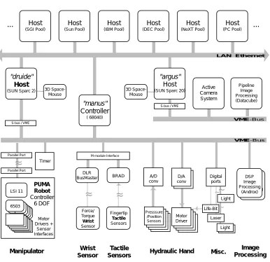
2.1 Actuation: The Puma Robot 11 ~ Host (Sun Pool) Host (SGI Pool) Host (IBM Pool) Host (NeXT Pool) Host (PC Pool) Host (DEC Pool)

~

motor driver DA conv VME-Bus Parallel Port LSI 11 6503 Motor Drivers + Sensor Interfaces PUMA Robot Controller 6 DOF Timer DLR

BusMaster BRAD

Force/ Torque Wrist Sensor Fingertip Tactile Sensors D/A conv A/D conv Digital ports motor driver motor driver Motor Driver motor driver motor driver motor driver Presssure /Position Sensors DSP image processing (Androx) DSP Image Processing (Androx) VME-Bus

Manipulator Wrist

Sensor

Tactile

Sensors Hydraulic Hand

Image Processing

LAN Ethernet

Pipeline Image Processing (Datacube)

~

M-module Interface Parallel Port S-bus / VME

"argus"

Host

(SUN Sparc 20)

"druide"

Host (SUN Sparc 2)

"manus" Controller ( 68040) 3D Space- Mouse 3D Space- Mouse

S-bus / VME

[image:25.595.86.472.113.487.2]

Active Camera System ... ... Laser Light Light Light ~ ~ Life-Bit Misc.

(26)

carry the required payload of about 3 kg and which can be turned into an

open, real-time robot, was found with a Puma 560 Mark II robot. It is

prob-ably “the” classical industrial robots with six revolute joints. Its geome-try and kinematics1 _{is subject of standard robotics textbooks (Paul 1981;}

Fu, Gonzalez, and Lee 1987). It can be characterized as a medium fast (0.5 m/s straight line), very reliable, robust “work horse” for medium pay loads. The action radius is comparable to the human arm, but the arm is stronger and heavier (radius 0.9 m; 63 kg arm weight). The Puma Mark II controller comprises the power supply and the servo electronics for the six DC motors. They are controlled by six parallel microprocessors and coordinated by a DEC LSI-11 as central controller. Each joint micropro-cessor (Rockwell 6503) implements a digital PD controller, correcting the commanded joint position periodically. The decoupled joint position control operates with 1 kHz and originally receives command updates (setpoints) every 28 ms by the LSI-11.

In the standard application the Puma is programmed in the interpreted language VAL II, which is considered a flexible programming language by industrial standards. But running on the main controller (LSI-11 proces-sor), it is not capable of handling high bandwidth sensory input itself (e.g., from a video camera) and furthermore, it does not support flexible control by an auxiliary computer. To achieve a tight real-time control directly by a Unix workstation, we installed the software package RCI/RCCL (ward and Paul 1986; Lloyd 1988; Lloyd and Parker 1990; Lloyd and Hay-ward 1992).

The acronym RCI/RCCL stands for Real-time Control Interface and Robot

Control C Library. The package provides besides the reprogramming of the

robot controller a library of commands for issuing high-level motion com-mands in the C programming language. Furthermore, we patched the Sun operating system OS 4.1 to sufficient real-time capabilities for serving a re-liable control process up to about 200 Hz. Unix is a multitasking operating system, sequencing several processes in short time slices. Initially, Unix was not designed for real-time control, therefore it provides a regular pro-cess only with timing control on a coarse time scale. But real-time propro-cess- process-ing requires, that the system reliably responds within a certain time frame. RCI succeeded here by anchoring the synchronous trajectory control task

1_{Designed by Joe Engelberger, the founder of Unimation, sometimes called the father}

(27)

2.1 Actuation: The Puma Robot 13 (a special thread) at a special device driver serving the interrupts from a

timer card. The control task is thus running independently and outside the planning task. By this means, sensory information (e.g. camera or force sensors) can be processed and feedback in a very effective and convenient manner.

For example, by default our DLR 6 D wrist sensor is read out about the currently exerted force and torque vector (3+3=6 D) between the robot arm and the robot hand (Fig. 2.1, 2.4). The DLR Force-Torque-Sensor (FTS) was developed by the robotics group of Prof. Hirzinger of the DLR, Oberpfaf-fenhofen, and is a spin-off from the ROTEX Spacelab mission D2 (Hirzinger, Brunner, Dietrich, and Heindl 1994). As indicated in Fig. 2.2, the FTS is an micro-controller based sensory sub-system, which communicates via a special field-bus with the VME-bus.

Force Control

Law

Guard Coordinate _transform

Coordinate transform

Position Controller

Coordinate transform

+ Gravity Compens. 1-S

S

+ -

Robot + Environment

Sensory Pattern

X_des

X_trans F_des

F_meas F_trans

X θdes

θmeas

[image:27.595.83.468.349.550.2]

(Sun "druide") (Puma Controller)

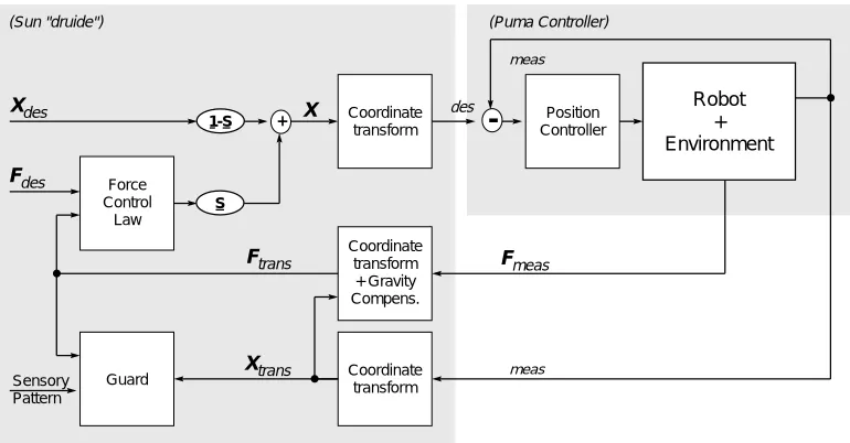
Figure 2.3: A two-loop control scheme for the mixed force and position control. The inner, fast loop runs on the joint micro controller within the Puma controller, the outer loop involves the control task on “druide”.

(28)

with environment interaction need quick response and therefore require, a very high frequency of the digital force control loop. The bottleneck is given by the Puma controller structure. The realizable force control in-cludes a fast inner position loop (joint micro controller) with a slower outer force loop (involving the Sun “druide”). But still, by generating the robot trajectory setpoints on the external Sun workstation, we could double the control frequency of VAL II and establish a stable outer control loop with 65 Hz.

Fig. 2.3 sketches the two-loop control scheme implemented for the mixed force and position control of the Puma. The inner, fast loop runs on the joint micro controller within the Puma controller, the outer loop involves the control task on the Sun workstation “druide”. The desired position

Xdesand forcesFdesare given for a specified coordinate system (here

writ-ten as generalized 6 D vectors: position and orientation in roll, pitch, yaw (see also Fig. 7.2 and Paul 1981)Xdes = (

p

x

p

y

p

z

)and generalized

forceFdes = (

f

x

f

y

f

z

m

x

m

y

m

z)). The control law transforms the force

deviation into a desired position. The diagonal selection matrix elements in S choose force controls (if 1) or position control (if 0) for each axis, fol-lowing the idea of Cartesian sub-space control2_{. The desired position is}

transformed and signaled to the joint controllers, which determine appro-priate motor power commands. The results of the robot - environment in-teractionFmeasis monitored by the force-torque sensor measurement and

transformed to the net acting force Ftrans after the gravity force

compu-tation. The guard block checks on specified sensory patterns, e.g., force-torque ranges for each axes and whether the robot is within a safe-marked work space volume. Depending on the desired action, a suitable controller scheme and sets of parameters must be chosen, for example, S, gains, stiff-ness, safe force/position patterns). Here the efficient handling and access of parameter sets, suitable for run-time adaptation is an important issue.

2_{Examples for suitable selection matrices are: S=diag(0,0,1,0,0,0) for a compliant}

mo-tion with a desired force inzdirection, orbS=diag(0,0,1,1,1,0) for aligning two flat

sur-faces (with surface normal inz). A free translation andz-rotational follow controller in

(29)

2.1 Actuation: The Puma Robot 15

(30)

2.2 Actuation: The Hand “Manus”

[image:30.595.162.318.332.555.2]

For the purpose of studying dextrous manipulation tasks, our robot lab is equipped with an hydraulic robot hand with (up to) four identical 3-DOF fingers modules, see Fig. 2.4. The hand prototype was developed and built by the mechanical engineering group of Prof. Pfeiffer at the Technical Uni-versity of Munich (“TUM-hand”). We received the final hand prototype comprising four completely actuated fingers, the sensor interface, and mo-tor driver electronics. The robot finger's design and its mobility resembles that of the human index finger, but scaled up to about 110 %.

Figure 2.5: The kinematics of the TUM robot finger. The car-danic base joint allows 15

side-wards gyring (

3) and full

ad-duction (

4) together with two

coupled joints (

5 =

6). (after

Selle 1995)

(31)

2.2 Actuation: The Hand “Manus” 17

2.2.1 Oil model

The finger joints are driven by small, spring loaded, hydraulic cylinders, which connect each actuator to the base station by a oil hose. In contrast to the more standard hydraulic system with a central power supply and valve controlled bi-directional powered cylinder, here, each finger cylin-der is one-way powered from a corresponding cylincylin-der at the base sta-tion. Unfortunately, the finger design does not foresee integrated sensors directly at the fingers.

Motor

X _m X _f

A_f A_m

k

Finger p

Base Station

pistonExt.

F

Oil Hose

[image:31.595.79.470.279.362.2]

κ

Figure 2.6: The hydraulic oil system.

The control system has to rely on indirect feedback sensing through the oil system. Fig. 2.6 displays the location of the two feedback sensors. In each degree of freedom (

i

) the piston position

x

m of the motor

cylin-der (linear potentiometer) and (

ii

)the pressure

p

in the closed oil system

(membrane sensor with semi-conductor strain-gauge) is measured at the base station. The long oil hose is not perfectly stiff, which makes this oil system component significantly expandable (4 m, large surface to volume ratio). This bears the advantage of a naturally compliant and damped sys-tem but bears also the disadvantage, that even pure position control must consider the force - position coupled oil model (Menzel et al. 1993; Selle 1995; Walter and Ritter 1996c).

2.2.2 Hardware and Software Integration

(32)

pro-cessor board. Following the example of RCCL, the “Manus Control C Library” (MCCL) was developed and implemented (Rankers 1994; Selle 1995). To facilitate an arm-hand unified planning level, the Unix work-station “druide” is set up to issue finger motion (piston, joint, or Cartesian position) and force control requests to the “manus” controller (Fig. 2.2).

Further Fingertip

Sensors Oil Model

Finger State Estimation +

- τ

-

Finger Cylinder

+ Environment

X_{f, des} F_{f, des}

K -1 _ControllerPD

DC Motor and Oil Cylinder

e

X_{f, estim} F_{f, estim}

X_m p

Oil System

F ext X

f

[image:32.595.137.514.224.348.2]

F friction

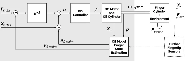
Figure 2.7:A control scheme for the mixed force and position control running on the embedded VME-CPU “manus”. The original robot hand design allows only indirect estimation of the finger state utilizing a model of the oil system. Certain kinds of influences, especially friction effects require extra information sources to be satisfyingly accounted for – as for example tactile sensors, see Sec. 2.3.

The achieved performance in dextrous finger control is a real challenge and led to the development of a simulator package for a more detailed study of the oil system (Selle 1995). The main sources of uncertainty are friction effects in combination with the lack of direct sensory feedback. As illustrated in Fig. 2.7, extra sensory information is required to fill this gap. Particularly promising are different kinds of tactile sense organs. The human skin uses several types of neural receptors, sensitive to static and dynamic pressure in a remarkable versatile manner.

In the following section extensions to the robot's senses are described. They are the prerequisite for more intelligent, semi-autonomous robotic systems. As already mentioned, todays robots are usually restricted to the proprioceptors of their actuator positions. For environment interac-tion two categories can be distinguished: (i) remote senses, which are

(33)

2.3 Sensing: Tactile Perception 19

2.3 Sensing: Tactile Perception

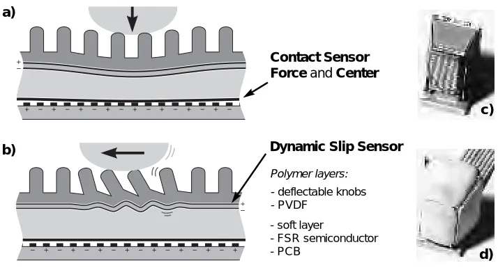
Despite the explained importance of good sensory feedback sub-systems, no suitable tactile sensors are commercially available. Therefore we fo-cused on the design, construction and making of our own multi-purpose, compound sensor (Jockusch 1996). Fig. 2.8 illustrates the concept, achieved with two planar film sensor materials: (i) a slow piezo-resistive FSR ma-terial for detection of the contact force and position, and (ii) a fast piezo-electric PVDF foil for incipient slip detection. A specific consideration was the affordable price and the ability to shape the sensors in the particular desired forms. This enables to seek high spatial coverage, important for fast and spatially resolved contact state perception.

Contact Sensor Force and Center

Dynamic Slip Sensor

Polymer layers:

- deflectable knobs - PVDF

- soft layer

- FSR semiconductor - PCB

a)

b)

c)

[image:33.595.98.455.333.527.2]

d)

Figure 2.8: The sandwich structure of the multi-layer tactile sensor. The FSR sensor measures normal force and contact center location. The PVDF film sensor is covered by a thin rubber with a knob structure. The two sensitive layers are separated by a soft foam layer transforming knob deflection into local stretching of the PVDF film. By suitable signal conditioning, slippage induced oscillations can be detected by characteristic spike trains. (c–d:) Intermediate steps in making the compound sensor.

(34)

on an object surface, see Jockusch, Walter, and Ritter (1996).

Efficient system integration is provided by a dedicated, 64 channel sig-nal pre-conditioning and collecting micro-computer based device, called “MASS” (= Multi channel Analog Signal Sampler, for details see Jockusch 1996). MASS transmits the configurable set of sensor signals via a high-speed link to its complementing system “BRAD” – the Buffered Random Access Driverhosted in the VME-bus rack, see Fig. 2.2. BRAD writes the time-stamped data packets into its shared memory in cyclic order. By this means, multiple control and monitor processes can conveniently access the most recent sensor data tuple. Furthermore, entire records of the re-cent history of sensor signals are readily available for time series analysis.

0 0.5 1 1.5 2 2.5 3 3.5 4

grip slide release

pulse output analog signal

force sensor readout

Time [s]

Force Readout FSR Preprocessing Output

Dynamic Sensor Analog Signal

Contact Sliding Breaking

Contact

Figure 2.9: Recordings from the raw and pre-processed signal of the dynamic slippage sensor. A flat wooden object is pressed against the sensor, and after a short rest tangentially drawn away. By band-pass filtering the slip signal of interest can be extracted: The middle trace clearly shows the sudden contact and the slippage phase. The lower trace shows the force values obtained from the second sensor.

(35)

2.4 Remote Sensing: Vision 21 These initial results from the new tactile sensor system are very

promis-ing. We expect to (i) fill the present gap in proprioceptive sensory infor-mation on the oil cylinder friction state and therefore better finger fine control; (ii) get fast contact state information for task-oriented low-level grasp reflexes; (iii) obtain reliable contact state information for signaling higher-level semi-autonomous robot motion controllers.

2.4 Remote Sensing: Vision

In contrast to the processing of force-torque values, the information gained by the image processing system is of very high-dimensional nature. The computational demands are enormous and require special effort to quickly reduce the huge amount of raw pixel values to useful task-specific infor-mation.

Our vision related hardware currently offers a variety of CCD cameras (color and monochrome), frame grabbers and two specialized image pro-cessors systems, which allow rapid pre-processing. The main subsystems are (i) two Androx ICS-400 boards in the VME bus system of “druide”(see Fig. 2.2), and (ii) A MaxVideo-200 with a DigiColor frame grabber exten-sion from Datacube Inc.

Each system allows simultaneous frame grabbing of several video chan-nels (Androx: 4, Datacube: 3-of-6 + 1-of-4), image storage, image oper-ations, and display of results on a RGB monitor. Image operations are called by library functions on the Sun hosts, which are then scheduled for the parallel processors. The architecture differs: each Androx system uses four DSP operating on shared memory, while the Datacube system uses a collection of special pipeline processors working easily in frame rate (max 20 MByte/s). All these processors and crossbar switches are register pro-grammable via the VME bus. Fortunately there are several layers of library calls, helping to organize the pipelines and their timely switching (by pipe altering threads).

(36)

However, the tremendous growth in general-purpose computing power allows to shift already the entire exploratory phase of vision algorithm development to general-purpose high-bandwidth computers. Fig. 2.2 ex-poses various graphic workstations and high-bandwidth server machines at the LAN network.

2.5 Concluding Remarks

We described work invested for establishing a versatile robotics hardware infrastructure (for a more extended description see Walter and Ritter 1996c). It is a testbed to explore, develop, and evaluate ideas and concepts. This investment was also prerequisite of a variety of other projects, e.g. (Littmann et al. 1992; Kummert et al. 1993a; Kummert et al. 1993b; Wengerek 1995; Littmann et al. 1996).

An experimental robot system comprises many different components, each exhibiting its own characteristics. The integration of these sub-systems requires quite a bit of effort. Not many components are designed as intel-ligent, open sub-systems, rather than systems by themselves.

Our experience shows, that good design of re-usable building blocks with suitably standardized software interfaces is a great challenge. We find it a practical need in order to achieve rapid experimentation and eco-nomical re-use. An important issue is the sharing and interoperating of robotics resources via electronic networks. Here the hardware architec-ture must be complemented by a software framework, which complies to the special needs of a complex, distributed robotics hardware. Efforts to tackle this problem are beyond the scope of the present work and therefore described elsewhere (Walter and Ritter 1996e; Walter 1996).

(37)

Chapter 3

Artificial Neural Networks

This chapter discusses several issues that are pertinent for the PSOM algo-rithm (which is described more fully in Chap. 4). Much of its motivation derives from the field of neural networks. After a brief historic overview of this rapidly expanding field we attempt to order some of the prominent network types in a taxonomy of important characteristics. We then pro-ceed to discuss learning from the perspective of an approximation prob-lem and identify several probprob-lems that are crucial for rapid learning. Fi-nally we focus on the so-called “Self-Organizing Maps”, which emphasize the use of topology information for learning. Their discussion paves the way for Chap. 4 in which the PSOM algorithm will be presented.

3.1 A Brief History and Overview

of Neural Networks

The field of artificial neural networks has its roots in the early work of McCulloch and Pitts (1943). Fig. 3.1a depicts their proposed model of an idealized biological neuron with a binary output. The neuron “fires” if the weighted sum P

j

w

ij

x

j (synaptic weights

w

) of the inputs

x

_j (dendrites) reaches or exceeds a threshold

w

_i. In the sixties, the Adaline (Widrow and Hoff 1960), the Perceptron, and the Multi-Layer Perceptron (“MLP”, see Fig. 3.1b) have been developed (Rosenblatt 1962). Rosenblatt demon-strated the convergence conditions of an early learning algorithm for the one-layer Perceptron. The learning algorithm described a way of itera-tively changing the weights.

(38)

Σ

wi1 wi2

wi3

yi x1

x2

x3

y1 x1

x2

x3 y2

1 1

wi

input layer

hidden layer

output layer a) b)

Figure 3.1: (a) The McCulloch-Pitts neuron “fires” (output

y

i=1 else 0) if the weighted sumP

j

w

ij

x

j of its inputs

x

j reaches or exceeds a threshold

w

i. If this binary threshold function is generalized to a non-linear sigmoidal transfer func-tion

g

(

P

j

w

ij

x

j;

w

i)(also called activation, or squashing function, e.g.

g

()=tanh()),

the neuron becomes a suitable processing element of the standard (b) Multi-Layer

(39)

3.1 A Brief History and Overview of Neural Networks 25 In (1969) Minsky and Papert showed that certain classes of problems,

e.g. the “exclusive-or” problem, cannot be learned with the simple percep-tron. They doubted that learning rules could be found for computation-ally more powerful multi-layered networks and recommended to focus on the symbolic oriented learning paradigm, today called artificial intelligence (“AI”). The research funding for artificial neural networks was cut, and it took twenty years until the field became viable again.

An important stimulus for the field was the multiple discovery of the error back-propagation algorithm. Its has been independently invented in several places, enabling iterative learning for multi-layer perceptrons (Werbos 1974, Rumelhart, Hinton, and Williams 1986, Parker 1985). The MLP turned out to be a universal approximator, which means that using a sufficient number of hidden units, any function can be approximated arbitrarily well. In general two hidden layers are required - for continuous functions one layer is sufficient (Cybenko 1989, Hornik et al. 1989). This property is of high theoretical value, but does not guarantee efficiency of any kind.

Other important developments where made: e.g. v.d. Malsburg and Willshaw (1977, 1973) modeled the ordered formation of connections be-tween neuron layers in the brain. A strongly related, more formal algo-rithm was formulated by Kohonen for the development of a topographi-cally ordered map from a general space of input stimuli to a layer of ab-stract neurons. We return to Kohonen's work later in Sec. 3.7.

Hopfield (1982, 1984) contributed a famous model of the content-addressable Hopfield network, which can be used e.g. as associative memory for im-age completion. By introducing an energy function, he opened the mathe-matical toolbox of statistical mechanics to the class of recurrent neural

net-works (mean field theory developed for the physics of magnetism). The

Boltzmann machine can be seen as a generalization of the Hopfield net-work with stochastic neurons and symmetric connection between the neu-rons (partly visible – input and output units – and partly hidden units). “Stochastic” means that the input influences the probability of the two possible output states (

y

2f;1

+1g) which the neuron can take (spin glass

like).

(40)

differences to other approaches are discussed in the next sections.

3.2 Network Characteristics

Meanwhile, a large variety of neural network types have emerged. In the following we present a (certainly incomplete) taxonomic ordering and point out several distinguishable axes:

Supervised versus Unsupervised and Reinforcement Learning: In super-vised learning paradigm, the training input signal is given with a pairing output signal from a supervisor or teacher knowing the cor-rect answer. Unsupervised networks (e.g. competitive learning, vec-tor quantization, SOM, see below) draw information from redundan-cies in the input data distribution.

An intermediate form is the reinforcement learning. Here the sys-tem receives a “reward” or “quality” signal, indicating whether the network output was more or less successful. A major problem is the meaningful credit assignment to the responsible network parts. The structural problem is extended by the temporal credit assignment problem if the quality signal is delayed and a sequence of decisions contributed to the overall result.

Feed-forward versus Recurrent Networks: In feed-forward networks the information flow is unidirectional from the input to the output layer. In contrast, recurrent networks also connect neuron outputs back as additional feedback inputs. This enables a network intern dynamic, controlled by the given input and the learned network characteris-tics.

(41)

uti-3.2 Network Characteristics 27 lize a form of recurrent network dynamic operating on a continuous

attractor manifold.

Hetero-association and Auto-association: The ability to evaluate the given input and recall the desired output is also called association.

Hetero-association is the common (one-way) input to output mapping

(func-tion mapping). The capability of auto-associa(func-tion allows to infer dif-ferent kinds of desired outputs on the basis of an incomplete pat-tern. This enables the learning of more general relations in contrast to function mapping.

Local versus Global Representation: For a network with local represen-tation, the output of a certain input is produced only by a localized

part of the network (which is pin-pointed by the notion of a

“grand-mother cell”). Using global representation, the network output is as-sembled of information distributed over the entire network. A global representation is more robust against single neuron failures. Here, as a result the network performance degrades gracefully, like the biological brain usually does. The local representation of knowledge is easier to interpret and not endangered by the so-called “catastrophic

inter-ference”, see “on-line learning” below.

Batch versus Incremental Learning: Calculating the network weight up-dates under consideration of all training examples at once is called “batch-mode” learning. For a linear network, the solution of this learning task can be shown to be equivalent to finding the pseudo-inverse of a matrix, that is formed by the training data. In contrast, incremental learning is an iterative weight update that is often based on some gradient descent for an “error function”. For good conver-gence this often requires the presentation of the training examples in a stochastic sequence. Iterative learning is usually more efficient, particularly w.r.t. memory requirements.

(42)

Consider the case of a network, which is already well trained with the data set A. When a new data set B gets available, the knowledge about “skill” A can be deteriorated (interference) mainly in the fol-lowing ways:

(i) due to re-allocation of the computational resources to new

map-ping domains the old skill (A) becomes less accurate (“stability –

plas-ticity” problem).

(ii) Further data sets A and B might be inconsistent due to a change

in the mapping task and require a re-adaptation.

(iii) Beyond these two principal, problem-immanent interferences, a global learning process can cause “catastrophic interference”: when

the weight update to new data is global, it is hard to control, how this influences knowledge previously learned. A popular solution is to memorize the old dataset A, and retrain the network based on the merged dataset A and B.

One of the main challenges in on-line learning is the proper control of the current context. It is crucial in order to avoid wrong general-ization for other contexts - analog to the human “traumatic experi-ences” (see also localized representations above, mixture-of-experts below and Chap. 9 for the problem of context oriented learning).

Fixed versus adaptable network structures As pointed out before, the suit-able network (model) structure has significant influence on the effi-ciency and performance of the learning system. Several methods have been proposed for tackling the combined problem of adapt-ing the network weights and dynamically decidadapt-ing on the structural adaptation (e.g. growth) of the network (additive models). Strategies on selecting the network size will be later discussed in Sec. 3.6.

For a more complete overview of the field of neural networks we refer the reader to the literature, e.g. (Anderson and E. Rosenfeld 1988; Hertz, Krogh, and Palmer 1991; Ritter, Martinetz, and Schulten 1992; Arbib 1995).

3.3 Learning as Approximation Problem

(43)

3.3 Learning as Approximation Problem 29 Usually, the process of learning is based on a certain amount of apriori

knowledge and a set of training examples. Its goal is two-fold:

the learner should be able to recognize the re-occurance of a

previ-ously seen situation (stimuli or input) and associate the correct an-swer (response or output) as learned before;

in new, previously un-experienced situations, the learner should

gen-eralizeits knowledge and infer the answer appropriately.

The primary problem of learning is to find an appropriate

representa-tion of the learned knowledge or skill: its input (stimuli) and output

(re-sponses). The reason is rather simple and fundamental: no system can learn, what it cannot represent.

We can distinguish three basic types of task describing variables

x

:

1. the orderable, continuous valued representations (e.g. length, speed, temperature, force) with a defined order relation (

x

_i

< x

_j) and an ex-isting distance metricj

x

i;

x

jj;

2. a periodic or circular variable representation (e.g. azimuth angles, hour of the day) with defined distance, but without a clear order relation (“wrap-around”; is Monday before or after Saturday?);

3. the symbolic and categorical representation

x

2 f

c

1

:::c

k

g, like

cities, attributes and generally names. Here, nor an order, neither a distance relation between

x

_iand

x

_j does exist, just the binary equiv-alence relation is defined (

x

_i =

x

j, or

x

i 6=

x

j).

Sometimes variables are represented depending on the context, e.g. “red” color may get coded as category, as circular hue value, or as orderable location in the color triangle.

A desired skill can be modeled as the mapping between an input space and an output space. The input space (later notated

X

in

(44)

Most methods prefer orderable, variables as input variables type (neu-ral nets), some others prefer categorical variables (artificial intelligence and machine learning approaches). Depending on the type of output vari-ables different frameworks offer methods called regression, approxima-tion, classificaapproxima-tion, system identificaapproxima-tion, system estimaapproxima-tion, pattern recog-nition, or learning. Tab. 3.1 compares names for learning task, common in different domains of research.

Output Type Continuous Values Symbolic Values vs. Framework Orderable Variables Categorical Variables

Neural Networks Learning Learning

Machine Learning Sub-symbolic & Fuzzy Learning Learning

Mathematics Approximation Quantization

Statistics Regression Classification

Engineering System Identification & Estimation Pattern Recognition

Table 3.1: Creating and refining a model in order to solve a learning task has various common names in different disciplines.

In the following we mainly focus on the variable type continuous and orderable. It can be considered as the most general case, since periodic variables (2) can transformed by the trick of mapping the phase infor-mation into a pair of sine and cosine values (of course the topology is unchanged). Categorical output values (3) are often prepared by a com-petitive component which selects the dominating component in a multi-dimensional output (“winner takes all”). It is interesting to notice, that

Fuzzy Systems work the opposite way. Continuous valued inputs are

ex-amined on their probability to belong to a particular class (fuzzy mem-bership). All combinations are propagated through a symbolic rule set (if-then-else type) and the output “de-fuzzificated” into a continuous out-put. The attractive point is the simplicity how to insert categorical “expert knowledge” into the system.

We consider a system that generates data and is presumed to be de-scribed by the multivariate function

f

(x) (possible perturbed by noise).

With continuous valued variables, the learning task is to model the system by the function

F

(w

x) that can serve as a reasonable approximation of

f

(45)

3.4 Approximation Types 31 training or design points

D

_trainwithin the domain of interest

D

_train

D

X

. xdenotes the input variable setx = f

x

1

:::x

d

g 2

X

,w a parameter

setw=(

w

1

w

2

:::

).

A good measure for the quality of the approximation will depend on the intended task. However, in most cases accuracy is of importance and is measured employing a distance function

dist

(

f

(x)

F

(w

x))(e.g. L2 norm).

The lack of accuracy or lack-of-fit

LOF

(

F

)is often defined by the expected

error

LOF

(

FD

)=h

dist

(

f

(x)

F

(w

x))iD (3.1)

the

dist

function averaged over the domain of interest

D

. The approx-imation problem is to determine the parameter set w

, that minimizes

LOF

(

FD

). The ultimate solution depends strongly on

F

. If it exists, it is

called “best approximation” (see e.g. Davis 1975; Poggio and Girosi 1990; Friedman 1991).

Summarizing, several main problems in building a learning system can be distinguished:

(i) encoding the problem in a suitable representationx;

(ii) finding a suitable approximation function

F

;

(iii) choosing the algorithm to find optimal values for the parameters

W

;

(iv) the problem of efficiently implementing the algorithm.

The proceeding chapter 4 will present the PSOM approach with respect to (ii)–(iv). Numerous examples for (i) are presented in the later chapters. The following section discusses several common methods for (ii)

3.4 Approximation Types

In the following we consider some prominent examples of approximat-ing functions

F

(w

x) : IRd ! IR – for the moment simplified to

one-dimensional outputs.

The classical linear case is

(46)

the dot product with inputx, usually augmented by a constant one.

This linear regression scheme corresponds to a linear, single layer net-work, compare Fig. 3.1.

The classical approximation scheme is a linear combination of a suitable set of basis functionsf

B

igon the original inputx

F

(w

x)=

m

X

i=1

w

i

B

i(x) (3.3)

and corresponds to a network with one hidden layer. This represen-tation includes global polynomials (

B

_i are products and powers of the input components; compare polynomial classifiers), as well as expansions in series of orthogonal polynomials and splines.

Nested sigmoids schemes correspond to the Multi-Layer Perceptron and can be written as

F

(w

x)=

g

0 @

X

k

u

k

g

0 @

X

j

v

kj

g

X

i

w

ji

x

i

!

! 1 A

1

A (3.4)

where

g

()is a sigmoid transfer function, and w = (

w

ji

v

kj

u

k

)

denote the synaptic input weights of the neural unit. This scheme of nested non-linear functions is unusual in the classical theory of approximation (Poggio and Girosi 1990).

Projection Pursuit Regression uses approximation functions, which are a sum of univariant functions

B

_i of linear combinations of the input variables:

F

(w

x)=

m

X

i=1

B

i(wix) (3.5)

The interesting advantage is the straight forward solvability for affine transformations of the given task (scaling and rotation) (Friedman 1991).

(47)

3.4 Approximation Types 33

σ

RBF

norm.

[image:47.595.83.464.133.334.2]

1

< <

σ

2

σ

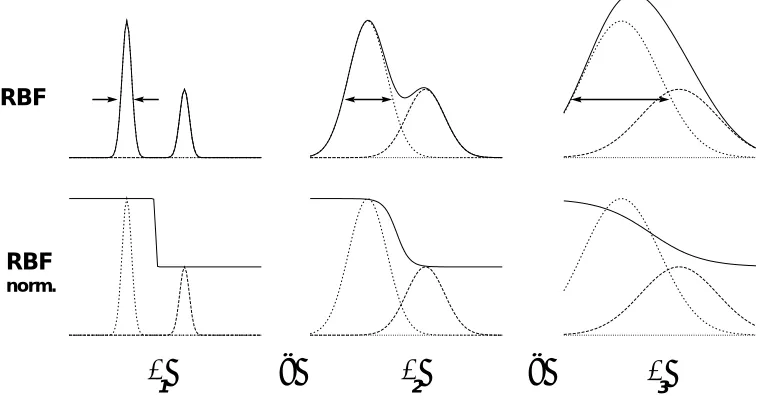
3

Figure 3.2: Two RBF units constitute the approximation model of a function. The upper row displays the plain RBF approach versus the results of the normal-ization step in the lower row. From left to right three basis radii

13 illustrate the

smoothing impact of an increasing

to distance ratio.

polynomial regression splines - but only for one or two components ofx(MARS algorithm (“Multivariate Adaptive Regression Splines”;

Friedman 1991).

Normalized Radial Basis Function (RBF) networks take the form of a weighted sum over reference pointswi located in the input space atwi:

F

(w

x)= P

i

(jx;uij)

w

i

P

i

(jx;uij)

(3.6)

The radial basis functions

: IR +

! IR +

usually decays to zero with growing argument and is often represented by the Gaussian bell function

(

r

) =

e

;(r= p

2) 2

, characterized by the width

(there-fore the RBF is sometimes called a kernel function). The division by the unweighted sum takes care on normalization and flat extrapo-lation as illustrated in Fig. 3.2. The learning is often split in two phases: (i) the placement of the centers is learned by an unsuper-vised method, for example by k-means clustering, learning vector

(48)

ad-hoc to the half mean distance of the base centers. The output val-ues

w

_i are learned supervised. The RBF net can be combined with a local linear mapping instead of a constant

w

_i (Stokbro, Umberger, and Hertz 1990), as described below. RBF network algorithms which generalize the constant sized radii

(sphere) to individually adapt-able tensors (ellipses) are called “Generalized Radial Basis Function networks” (GRBF), or “Hyper-RBF” (see Powell 1987; Poggio and Girosi 1990).

1 2

3 4

[image:48.595.221.415.271.360.2]

x

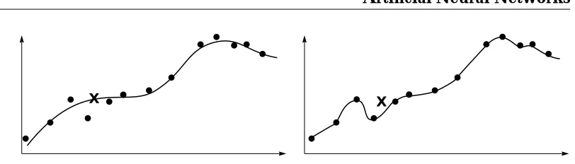
Figure 3.3: Distance versus topological distance. Four RBF unit center pointsui

(denoted 1

:::

4) around a test pointx(the circles indicate the width

).

Account-ing only for the distance jx;uij, the RBF output (Eq. 3.6) weights u

1 stronger

thanu

4. Considering the triangles spanned by the points 123 versus 234 reveals

thatxis far outside the triangle 123, but in the middle of the triangle 234.

There-fore,xcan be considered closer to point 4 than to point 1 — with respect to their

topological relation.

Topological Models and Maps are schemes, which build dimension re-ducing mappings from a higher dimensions input space to a low-dimensional set. A very successful model is the so-called “feature map” or “Self-Organizing Map” (SOM) introduced by Kohonen (1984) and described below in Sec. 3.7. In the presented taxonomy the SOM has a special role: it has a localized knowledge representation where the location in the neural layer encodes topological information beyond Euclidean distances in the input space (see also Fig. 3.3). This means that input signals which have similar “features” will map to neigh-boring neurons in the network (“feature map”). This topological pre-serving effect works also in higher dimensions (famous examples are Kohonen's Neural Typewriter for spoken Finnish language, and the

(49)

3.5 Strategies to Avoid Over-Fitting 35 could be extracted from a sequence of three-word sentences

(Koho-nen 1990; Ritter and Koho(Koho-nen 1989). The topology preserving prop-erties enables cooperative learning in order to increase speed and ro-bustness of learning, studied e.g. in Walter, Martinetz, and Schulten (1991) and compared to the so-called Neural-Gas Network in Walter (1991) and Walter and Schulten (1993).

The Neural-Gas Network shows in contrast to the SOM not a fixed grid topology but a “gas-like”, dynamic definition of the neighbor-hood function, which is determined by (dynamic) ranking of close-ness in the input space (Martinetz and Schulten 1991). This results in advantages for applications with inhomogeneous or u