Optimized Terminal Current Calculation
for Monte Carlo Device Simulation
P. D. Yoder, K. G¨artner, Ulrich Krumbein, and Wolfgang Fichtner,
Fellow, IEEEAbstract— We present a generalized Ramo–Shockley theorem (GRST) for the calculation of time-dependent terminal currents in multidimensional charge transport calculations and simula-tions. While analytically equivalent to existing boundary inte-gration methods, this new domain inteinte-gration technique is less sensitive to numerical error introduced by calculations of finite precision. Most significantly, we derive entirely new optimized formulas for the ensemble Monte Carlo estimation of steady-state terminal currents from the time-independent form of our GRST, which are in general not equivalent to the time-average of the true time-dependent terminal currents. We then demonstrate, both analytically and by means of example, how our new variance-minimizing terminal current estimators may be exploited to improve estimator accuracy in comparison to existing methods.
I. INTRODUCTION
T
HE simplest method which may be used to calculate terminal currents within Monte Carlo charge transport simulations is particle counting. That is, every particle which enters or leaves a contact is tallied as flux through that contact. This type of estimator tends to converge very slowly because of the relative rarity of boundary crossing events, a problem which is exacerbated by modern highly doped contacts in which the mean carrier velocity is only a small fraction of the thermal velocity. An analogous problem arises in moment-based simulation methods from the errors asso-ciated with numerical differentiation in highly doped contact regions [1], [2]. Simply displacing the boundary surface along which contact current is calculated outwards from the high doping regions can provide a partial solution for moment-based simulation in some circumstances [3], but does not fully address the fundamental problem for particle-based Monte Carlo simulations. Considerably better convergence may be obtained by calculating the exact instantaneous current densi-ties and and integrating this result along the contact boundary. This method, although very straightforward, has the disadvantage of relying heavily on the accuracy of the numerical solution on only a few grid nodes. Furthermore, as we will see, if steady-state terminal currents are our goal, there are better Monte Carlo estimators than the time-average of the true terminal currents. We offer a brief historical digression to motivate these thoughts.The original domain integration method for terminal cur-rents comes from the work of Shockley [4] and Ramo [5]
Manuscript received June 7, 1995; revised October 14, 1995. This paper was recommended by Associate Editor Duvall.
The authors are with the Swiss Federal Institute of Technology, In-tegrated Systems Laboratory, CH-8092 Z¨urich, Switzerland (e-mail: [email protected]).
Publisher Item Identifier S 0278-0070(97)09239-7.
based on a Green’s function technique. The Ramo–Shockley theorem has since been restated for multiple charge carriers [6] based on the linearity of Maxwell’s equations and separately using energy balance arguments. For the total current through contact , the final result is [4]–[6]
(1) where the summation is over all charges within the domain and and are the velocity vector, position vector, and the charge of the th particle, respectively. is the electric field generated by removing all charges from the domain and grounding all contacts except for contact which is set to 1 V. Although this result was derived under the as-sumption of constant contact potentials, an additional term may be added to (1) to account for their time dependence [7]. By integrating particle velocity over the entire device domain, the Ramo–Shockley theorem overcomes the previously mentioned numerical weakness of boundary integration schemes. In the general case of transients and/or generation/recombination processes, however, the Ramo–Shockley theorem offers no straightforward way to distinguish between the electron, hole, and displacement contributions to the total terminal current. It will easily be seen that the Ramo–Shockley domain integral formulation of terminal currents is a special case of a more general technique introduced by Mock [8] and Gajewski [9] based on the concept of “weak solutions,” which may be used to overcome this disadvantage. In the following analysis, we make use of this test function method to derive general expressions for the time-dependent electron, hole, displacement, and total current at arbitrary contacts.
We show that the time-independent form of these general-ized Ramo–Shockley theorem (GRST) expressions leads to a new class of estimators for steady-state terminal current, not generally equivalent to the time-average of the true terminal currents. We then derive the defining equations for a set of optimized test functions which, in conjunction with the new terminal current estimator formulas, lead to minimum-variance estimators for steady-state terminal currents in en-semble particle-based simulation. Finally, we provide an appli-cation of our method demonstrating its improved convergence properties.
II. GENERALIZED RAMO–SHOCKLEYTHEOREM
From the Poisson and Boltzmann transport equations, we have on the Lipschitzian domain
(2)
(3) (4) Current relations are in general . The symbol denotes ensemble average, and the variables , and are the electron and hole densities and the electrostatic potential. The symbols refer to the dielectric permittivity, time, space coordinate vector, funda-mental electronic charge, and net ionized impurity number density, respectively.
Differentiation of (4) with respect to time yields another equation which involves displacement current
(5) For each of the currents and , we have an equation of the form
(6) where denotes the total current. Let denote the usual Hilbert spaces and let and be a set of suitable test functions
(7) The boundary may consist of both Neumann and Dirichlet parts, , with and having positive surface measure. Multiplication of each equation of type (6) by the test function yields by integration by parts [8], [9]
(8) The choice of ensures that the surface integral at the right-hand side is the surface integral over the contact current (due to ). A similar test function technique has already found application in the calculation of capacitances in complex wiring structures [10].
From (2), (3), (5), and (8), the following simple equations result for the terminal currents at an arbitrary contact :
(9)
(10)
(11) (12) for which we wish to emphasize that the choice of test functions for each of the four above equations may be made
independently. This set of equations provides a powerful tool for examining the various contributions to each of the time-dependent terminal currents for multidimensional device topologies.
That the identity holds in general for (9)–(12) is a result of the properties of solutions to the defining transport equation, rather than a direct consequence of (9)–(12) themselves. Importance sampling schemes for particle-based simulation, which often “microscopically” disturb conserva-tion laws implicit in transport equaconserva-tions, may also disturb the identity if particle redistribution is performed between evaluations of any of the terminal current formulas.
III. REDUCTION OF NUMERICAL ERROR INMOMENT-BASED SIMULATION
Gajewski’s implementation of test functions took the fol-lowing form:
(13)
and is defined as
with defined as the unit step function, and defined as a third-degree polynomial. Note the similarity between De Visschere’s in (1) and above. Gajewski’s actual test functions , however, are more generally useful for purposes of numerical simulation due to their vanishing gradient near contact regions for , and their smoothness arising from the properties of . While one can most often choose a for which this technique eliminates contributions to the terminal currents from undesired regions, it may also simultaneously neglect useful regions. Working in the context of total current, Mock [8] proposed another defining equation
(14)
where is the electrical conductivity plus . This form involves no adjustable parameter and its solution exhibits qualitatively good properties for application in moment-based simulation.
IV. STEADY-STATE TERMINAL CURRENTESTIMATORS
General expressions for steady-state terminal currents may be derived from (9)–(12) by taking their expectation values with respect to time, setting all time derivatives equal to zero
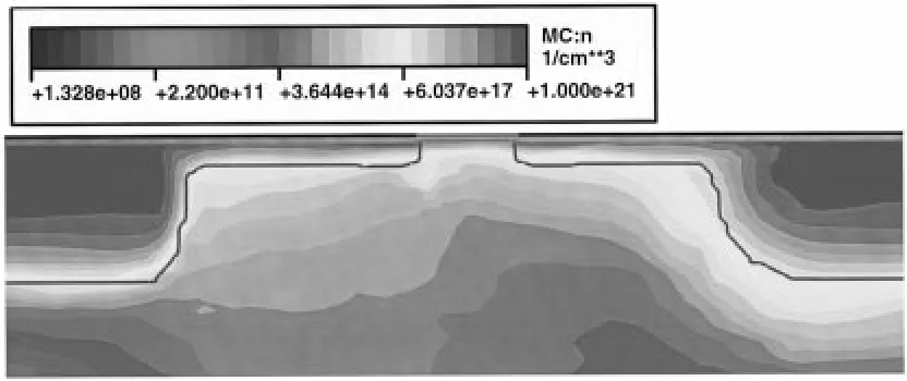
Fig. 1. Simulated free electron density for a 40-nm LDD NMOS transistor.
Fig. 2. Scalar electron current density variance tensor in units of 2:56 3 1004A2/cm4.
(17) (18)
In particle-based simulation, one may employ the following unbiased estimators for the steady-state terminal currents:
(19) (20) (21)
where and are the estimators for steady-state electron and hole current densities, and generation rates, respectively. It is important to keep in mind that although the choice of test functions in (9)–(12) and (15)–(18) influence the results only to the extent of the numerical precision of the calculation, the same is not true for (19)–(21), in which the choice of test functions plays a critical role. This is because the transport quantities in the integrands of the former groups of equations represent exact solutions of the time-dependent
and time-independent defining transport equation, whereas the corresponding quantities in the integrands of the latter group of equations are merely time-averaged estimates from ensemble simulation.
V. OPTIMIZATION OF TEST FUNCTIONS FOR
STEADY-STATE MONTECARLOTERMINAL CURRENT
The spatial convergence of Monte Carlo estimators is typi-cally far from uniform. This is due to a myriad of different fac-tors including: 1) spatially inhomogeneous fields; 2) thermal gradients; 3) inhomogeneity in material composition, doping level, or strain; or 4) importance sampling and other particle weighting/redistribution techniques. For the case of ensemble simulation, the spatial accuracy of the initial solution is often quite nonuniform. Making use of this fact, we minimize the variance of (19)–(21), , with respect to the test functions . Under the assumption of weak interparticle correlation, the resulting set of Euler–Lagrange equations is
[image:3.612.96.507.265.438.2]Fig. 3. Test function for electron drain current evaluation.
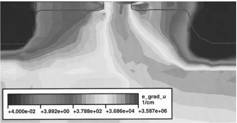
Fig. 4. Magnitude of the test function gradient.
(23) (24)
(25) For simulations using the generation/recombination estimator described in [11] and [12], the terms in (22) and (23) may in most circumstances be dropped. The quantity
is the position-dependent current density variance tensor. Although its exact form for a given problem requires numerical calculation, one may identify the following useful analytical approximation:
(26)
which might also be approximated for convenience by the scalar
(27) The symbols and are the charge density, thermal velocity, and mean velocity, respectively, for particles of type . and are the grid-dependent mean type-particle number and momentum relaxation time. The optimized terminal current estimators for steady-state simulation may then be written as
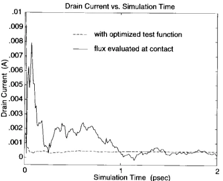
Fig. 5. Drain current convergence time comparison. The simulation was seeded with initial conditions close to the final solution.
It should be kept in mind that solutions of (22)–(24) always yield valid test functions for unbiased estimators in (28)–(30), independent of the exact form of . Note also that all solutions of the Poisson-like equation
(of which (24) and the simplified forms of (22) and (23) are limiting cases) with the boundary conditions of (25) automatically satisfy the condition , which is a sufficient condition for global current conservation
, in both the time-dependent and time-independent forms of the GRST. We further note that in the limit of homogeneous estimator convergence, the function reduces to the solution of the homogeneous Poisson equation, in which case (30) is exactly equivalent to the time-average of the original Ramo–Shockley formula (1).
VI. EXAMPLE: LDD NMOS DEVICE
We provide as a simple example, results for the the case of a 40-nm -channel LDD MOSFET, with gate and drain contacts set to 2 V with respect to the source and substrate contacts. A full-band ensemble Monte Carlo charge transport simulation was performed with the simulator Degas [11]. Fig. 1 shows the simulated electron density profile of the LDD device. A scalar version of (24) for the optimized test function was solved using the approximation to the current density variance tensor given by (27), whose solution was then employed in (28) to obtain the terminal currents. This scalar current density variance function is shown in Fig. 2. Figs. 3 and 4 show the test function solution of (24) and its gradient, respectively, the latter of which may be interpreted as a weighting function for the current density. Generally speaking, the greatest contributions to the current estimator come from regions of relatively low density and high mean velocity. Although the degree of improvement over competing techniques is of course example-dependent, we show a comparison of drain current estimator convergence time in Fig. 5, demonstrating the advantage of the optimized test function domain integration technique. In this example, both curves depict cumulative time-averaged data.
VII. CONCLUSIONS
We have presented a general domain integration method for calculating terminal currents in semiconductor devices, which avoids certain numerical problems associated with evaluating currents along boundary surfaces. This generalized form of the Ramo–Shockley theorem has the advantage of validity in the presence of generation/recombination processes, and one may easily distinguish between electron, hole, and displacement current contributions to the total current. Building upon the time-independent form of these expressions, we have pre-sented and demonstrated a variance-minimizing estimator for the calculation of steady-state terminal currents in ensemble Monte Carlo simulation, offering considerable improvement in estimator accuracy with respect to previous methods, which merely time-average the true terminal currents.
ACKNOWLEDGMENT
The first author would like to thank S. Laux for many insightful discussions.
REFERENCES
[1] B. S. Polsky and J. S. Rimshans, “Numerical simulation of transient processes in 2-D bipolar transistor,” Solid State Electron., vol. 24, pp. 1081–1085, 1981.
[2] E. Palm and F. Van de Wiele, “Current lines and accurate contact current evaluation in 2-D numerical simulation of semiconductor devices,” IEEE
Trans. Electron Devices, vol. ED-32, pp. 2052–2059, 1985.
[3] DESSIS0ISEManual, ISE Integrated Systems Engineering AG, Z¨urich,
Switzerland, 1994.
[4] W. Shockley, “Currents to conductors induced by a moving point charge,” J. Appl. Phys., vol. 9, pp. 635–636, 1938.
[5] S. Ramo, “Currents induced by electron motion,” Proc. IRE, vol. 27, pp. 584–585, 1939.
[6] P. De Visschere, “The validity of Ramo’s theorem,” Solid State
Elec-tron., vol. 33, pp. 455–459, 1990.
[7] H. Kim, H. S. Min, T. W. Tang, and Y. J. Park, “An extended proof of the Ramo–Shockley theorem,” Solid State Electron., vol. 34, pp. 1251–1253, 1991.
[8] M. S. Mock, Analysis of Mathematical Models of Semiconductor
De-vices. Dublin, Ireland: Boole, 1983.
[9] A. Gajewski, private communications; see also TOSCA Users Manual, Karl Weierstrass Institute, Berlin, Germany.
[10] W. E. Matzke, K. G¨artner, and B. Heinemann, “2-D and 3-D capacitance calculations for VLSI structures using the energy method,” in Simulation
of Semiconductor Devices and Processes, vol. 3, G. Baccarani and M.
Rudan, Eds., 1988, pp. 613–624.
[11] DEGAS0ISEReference Manual, ISE Integrated Systems Engineering
AG, Z¨urich, Switzerland, 1994.
[12] J. Gyoyoung, E. C. Kan, and R. W. Dutton, “A new practical method to include recombination-generation process in self-consistent Monte Carlo device simulation,” in Proc. 1996 Int. Conf. Simulation of Semiconductor
Processes and Devices, 1996, pp. 61–62.
P. D. Yoder received the B.S.E.E. degree from
Cornell University, Ithaca, NY, in 1989 and the M.S. and Ph.D. degrees in electrical engineering from the University of Illinois, Urbana, in 1991 and 1993, respectively.
K. G¨artner studied theoretical physics in Dresden,
Germany, and received the Ph.D. degree in nuclear reactor physics.
After working ten years in the field of neutron transport, he joined the Karl-Weierstraß-Institute for Mathematics in Berlin, Germany, in 1982. Since this time, his main interest has been in numerical prob-lems connected to PDE’s and semiconductor device models. In 1992, he joined the Interdisciplinary Center for Supercomputering at the ETH, Z¨urich, Switzerland, and since 1994 has been working with Professor W. Fichtner at the ETH Integrated Systems Lab.
Ulrich Krumbein received the Diploma in physics
from the University of Kaiserslautern, Germany, in 1990. He joined the Integrated Systems Laboratory at the ETH, Z¨urich, Switzerland, in 1990, where he earned the Ph.D. degree in semiconductor device simulation in 1997.
He is currently devoloping high-frequency MOS-FET’s at Siemens, Munich, Germany.
Wolfgang Fichtner (F’90) received the Dipl. Ing.
degree in physics and the Ph.D. degree in electrical engineering from the Technical University of Vi-enna, Austria, in 1974 and 1978, respectively.
From 1975 to 1978, he was an Assistant Professor in the Department of Electrical Engineering, Techni-cal University of Vienna. From 1979 through 1985, he worked at AT&T Bell Laboratories, Murray Hill, NJ. He has been Professor and Head of the Integrated Systems Laboratory at the Swiss Federal Institute of Technology (ETH), Z¨urich, Switzerland, since 1985. In 1993, he founded ISE Integrated Systems Engineering AG, a company in the field of technology CAD.