EHD augmentation of convective boiling within a transparent heat exchange

EHD Augmentation of Convective Boiling within

a Transparent Heat Exchanger

Gerard Joseph McGranaghan BSc, BA BAI

Department of Mechanical and Manufacturing Engineering Parsons Building

Trinity College Dublin 2

Ireland

I declare that I am the author of this thesis and that all work described herein is my own, unless otherwise referenced. Furthermore, this work has not been submitted, in whole or part, to any other university or college for any degree or qualification.

I authorize the library of Trinity College, Dublin to lend or copy this thesis.

________________________

This work investigated the influence of electrohydrodynamic forces on the two-phase flow patterns of HFE7000 refrigerant under convective boiling conditions. A flow loop was constructed which featured two novel transparent heat exchanger designs which facilitated visualisation of the flow field under EHD and diabatic conditions. In both designs, a sapphire tube was employed which allowed heat transfer and optical access to the boiling refrigerant. A stainless steel rod within the sapphire tube formed a high voltage electrode, while a thin layer of Indium Tin Oxide (ITO), deposited on the tube exterior provided an optically transparent though electrically conductive transparent ground. High-speed video imaging was combined with thermal-hydraulic measurements to relate flow patterns with voltage.

In Test Section A, the sapphire tube was surrounded by an acrylic channel through which heated water flowed, forming a transparent concentric heat exchanger. Heat transfer coefficients were calculated using thermocouples embedded in the sapphire tube wall and along the water side, and pressure drop was measured across the test section. A high speed camera recorded imagery along the test section length.

In the first study, experiments were carried out at a refrigerant mass flux (G) of 100 kg/m2_{s, inlet qualities from 0-45%, heat input (Q}//_{) of 12.4 kW/m}2 _{and EHD voltage} levels between 0 to 8 kV at 60Hz AC. It was found that at a constant heat flux of 12.4 kW/m2_{, EHD increased the heat transfer coefficients but with lower superheat} temperatures. At 2% inlet quality an EHD voltage of 8 kV altered the flow regime from a stratified flow with nucleate boiling to a complex mixed flow with oscillating bubbles and liquid jets, resulting in improved heat transfer. It was also found that as quality increased, EHD voltages precipitated a flow regime change from stratified to annular, resulting in improved heat transfer.

As the voltage rose to between 3 to 6 kV, a new flow regime where occurred where liquid was extracted from the lower layer towards the electrode. Bubble diameter and oscillation increased further. At 6 kV the flow alternated between oscillatory entrained bubble flow and a flow of waves of cresting bubbles and liquid. These cresting events caused wetting of the top of the tube. EHD forces seemed to contribute to the upward movement and cresting of the large bubbles. This regime accounted for around 55% of the total heat transfer enhancement.

At 7 kV another change appeared where liquid jets were produced and the flow began to alternate between the oscillating bubble and thin film regimes. In-tube flow was highly mixed, featuring droplets both from liquid jets and from bursting of the elongated bubbles. The top wall was highly wetted by the bubble bursting and cresting and this regime contributed 37% of the total heat transfer enhancement.

Firstly I want to express my sincere thanks and admiration to my supervisor Dr. Tony Robinson for all his guidance, patience, enthusiasm, understanding, and never ending stream of ideas. I am continually amazed by his profound knowledge of heat transfer, his ability to define the nub of a problem, and his optimism and ingenuity in finding alternative solutions whenever a plan didn’t work out. Working with him has been rewarding and a privilege.

I would like to thank Gerry Byrne in the Thermo lab for all his assistance with my ever-expanding test rig and his problem solving ability. Thanks are due to Mick Reilly and the Mechanical Workshop staff, Alex, Gabriel, JJ and Sean for their high quality work and for allowing me to work as one of them. I wish to also acknowledge the other departmental staff who contributed in various ways including Dr. Darina Murray and Dr. Tim Persoons. I am pleased to thank the intelligent and diligent visiting students from INSA Lyon, Aurelie Michel, Thomas Lebreton and Elodie Decourchelle who assisted so much with the design and experimental phases.

It would be a great slight if I wasn’t to mention my office mates, Alan, Brian, Rayhaan, Seamus and Tom, and also Stephen, Jessica and Karl. Without all their constant distractions, coffee, tea, poker, and lunchtime movies, I feel I might have been finished this thesis sooner, but it would not have been as much fun. Despite our different tastes in taste, and views on the volume it should be played, I hope we remain friends for life.

month when I worked on the EHD rig in McMaster University, they remained in correspondence when I was back in Ireland. My thanks also go to Dr. Roger Kempers for his valuable assistance in thermometry.

My gratitude is also due to a seasoned Mechanical Engineer, Mr. Tom Weymes whose gimlet eye scrutinised the thesis draft. I also want to thank most sincerely Dr. Michael Maguire for his tireless encouragement, patience, and assistance in the structure of the thesis, but most significantly, his unwavering friendship.

Declaration... i

Acknowledgements ... i

Table of Contents ... iii

List of Figures ... vi

List of Tables ... xiii

Nomenclature ... xiv

Latin Symbols ... xiv

Dimensionless Numbers ... xvi

Greek Symbols ... xvii

Chapter 1: Introduction ... 1

1.1 Motivations for Two-Phase Heat Transfer Augmentation... 1

1.1.1: Heat exchanger basics ... 1

1.1.2: Active Heat Transfer Augmentation ... 2

1.1 Enhancement of Heat Transfer by Electrohydrodynamics ... 3

1.2: Objectives of the Research ... 4

1.3: Outline of Thesis ... 4

1.4: Thesis Contributions ... 6

Chapter 2: Electrohydrodynamically Augmented Two-Phase Flow ... 9

2.1: Two Phase Flow... 9

2.1.1: Upward Vertical Flow ... 13

2.1.2: Horizontal Flow ... 14

2.1.3: Single Phase Heat Transfer Correlations ... 16

2.3: Relevant Studies in EHD Augmented Two-Phase flow ... 50

2.3.1: Electric Field Effects ... 53

2.4: Summary ... 60

Chapter 3: Experimental Facility and Methodology ... 61

3.1: Experimental Facility: The Test Rig ... 61

3.1.1: The Primary Loop ... 64

3.1.2: The Secondary Water Loops ... 66

3.1.3: Test Sections Used ... 67

3.1.4: The Cooling Loop ... 74

3.1.5: Expansion Vessel and Venting Arrangements ... 74

3.1.6: The Electrode and High Voltage Supply ... 75

3.2: Use of the ITO Coated Sapphire Tube ... 76

3.2.1: Thermal Conductivity Considerations of the Sapphire Tube ... 77

3.2.2: Surface Finish of the Tube. ... 78

3.2.3: Variation in thickness of the ITO coating. ... 79

3.3: The Data Acquisition System... 79

3.4: High Speed Imaging System ... 83

3.5: Experimental Procedure ... 84

3.6: Experimentally Measured Parameters and Test Conditions ... 86

3.7: Data Reduction ... 91

3.7.1: The Averaged Heat Transfer Coefficient ... 91

3.7.2: Data reduction for the Ohmically Heated Test Section B ... 92

3.8: Instrumentation Accuracy and Experimental Uncertainty ... 94

3.9: Energy Balance of Rig Heat Exchangers ... 97

3.10: Summary ... 101

Chapter 4: Experimental Results ... 103

4.1: Constant heat input and the influence of inlet quality... 103

4.1.1: Field Free Flow Patterns Observed and Comparison with Flow Pattern Correlations ... 104

4.1.5: Results for xin = 30% and G=100 kg/m2_{s ... 146}

4.1.6: Results for xin = 45% and G=100 kg/m2_{s ... 153}

4.1.7: Summary of Section 4.1... 161

4.1.8: Assessing EHD enhancement and penalty... 162

4.2: Heat Transfer Augmentation at Constant Inlet Temperature – Experimental Results and Discussion ... 164

4.2.1: Overview of Results at Constant Inlet Temperature ... 165

4.2.2: Field-free thermal hydraulics ... 166

4.2.3: EHD-augmented thermal hydraulics ... 170

4.2.4: EHD Enhancement ... 180

4.2.5: Application of PID control to flow loop ... 183

4.2.6: Summary of Section 4.2... 184

4.3: Heat Transfer Augmentation with Ohmic Heating - Experimental Results and Discussion ... 186

4.3.1: Aims of this Section ... 186

4.3.2: Comparison between 0 kV and 8 kV at the entry region ... 195

4.3.3: Comparison between 0 kV and 8 kV at the exit region ... 201

4.3.4: Comparison between 0 kV and 8 kV at x/L=⅜ and x/L=⅝ ... 207

4.3.5: Discussion of the Ohmically Heated Test Section Results ... 212

4.3.6: Differences between Water heated and Ohmically Heated Test Sections . 215 4.3.7: Summary of Section 4.3... 216

Chapter 5: Conclusions and Future Work ... 219

5.1: Summary of Work Completed ... 219

5.1.1: Summary of Chapters 1-3 ... 219

5.1.2: Summary of Chapter 4 ... 220

5.2: Conclusions ... 224

5.3: Recommendations for Further Study ... 226

References ... 227

Figure 1: Idealised model of two-phase flow in an inclined tube, adapted from Carey

[14] ... 10

Figure 2: Flow regimes in vertical upward co-current gas/liquid flow ... 13

Figure 3: Flow regimes as observed in horizontal co-current gas liquid flow. ... 15

Figure 4: Variation of convective boiling heat transfer coefficient with flow regime, adapted from Kreith and Boehm [18] ... 18

Figure 5: Vertical tube flow pattern map by Fair [20] ... 19

Figure 6: Flow regime map proposed by Hewitt and Roberts [21] ... 20

Figure 7: Baker flow map for horizontal tubes ... 21

Figure 8: Taitel and Dukler Two-phase Flow Pattern Map, from [20] ... 24

Figure 9: Hashizume two-phase flow map[26] ... 25

Figure 10: Flow map form as proposed by Steiner ... 26

Figure 11: Flow map of Kattan, Thome and Favrat [28], sourced from [28] ... 27

Figure 12: Typical two-phase flow patterns dependent on mass flux and quality overlaid on a Kattan et al. type flow map [20] ... 28

Figure 13: Flow map of Wojtan, Ursenbacher and Thome, image from [31] ... 29

Figure 14: Chart of Shah correlation, image from [33] ... 31

Figure 15: Steiner-Taborek description of boiling processes in a vertical tube ... 34

Figure 16: Simplified flow structures proposed in Kattan Thome Favrat Model, adapted from [20, 30] ... 37

Figure 17: Simulation of Wojtan et al. model showing heat transfer coefficient predictions and smooth transition between flow regime boundaries , image from [20] ... 42

Figure 18: Electric body force density components on a (a) charged body (b) neutral molecule (c) interface (d) bubble or droplet. Figure adapted from Bryan [48]... 47

Figure 19: The relationship between EHD number and Reynolds number ratio as a function of current for R134a, image from [5] ... 48

Figure 22: Flow pattern reconstructions proposed by Cotton for increasing DC voltage

levels (G = 100 kg/m2 _{s, q″=10 kW/m}2_{, and xin = 0%), image from [5] ... 55}

Figure 23: Flow map proposed by Cotton et al [5] ... 56

Figure 24: Illustrative representation of the various steps in the development and decay of the twisted liquid cone structures, image adapted from Ng [75] ... 58

Figure 25: Schematic of flow loop... 62

Figure 26: One of two heater units which together comprise DIR1 ... 64

Figure 27: Location of 0.5mm deep pockets in sapphire tube wall ... 68

Figure 28: Polypropylene supports, O-ring seal and gland ... 69

Figure 29: Miniature Type-T thermocouple with sealing gland ... 69

Figure 30: Sapphire tube and perspex jacket showing location of thermocouples ... 70

Figure 31: Test section showing developing length, sapphire tube, perspex jacket and polypropylene support pieces ... 71

Figure 32: Test section close up showing perspex jacket, sapphire tube, ground connection, SEC2 water outlet, one jacket thermocouple, and two sapphire wall thermocouples. ... 71

Figure 33: Schematic of rig with Test Section B ... 72

Figure 34: Electrical schematic of Test Section B ... 73

Figure 35 : Image of the second test section fitted with thermocouples ... 74

Figure 36: Electrode location in polypropylene supports (a) entrance and (b) exit ... 75

Figure 37: Conductive adhesive ring and copper earthing clamp ... 76

Figure 38: (a) Control cabinet, high voltage amplifier (b) datalogging hardware ... 80

Figure 39: Front panel of Labview® data acquisition program... 82

Figure 40: T-h diagram of HFE7000 ... 89

Figure 41: Electrical direct heater (DIR1) energy balance ... 97

Figure 42: HEX1 energy balance ... 98

Figure 43: Energy balance for test section ... 99

Figure 44: Energy balance for HEX3 (condenser) ... 100

water heated test section ... 107

Figure 49: Averaged HTC in the tube versus inlet quality over a range on inlet qualities from 2% to 45%, G=100kg/m2_{s, Q=150 W ... 108}

Figure 50: Flow regimes at locations x/L=⅛, ⅜, ⅝ & ⅞ at 0 kV, xin = 2% ... 109

Figure 51: Flow regimes at locations x/L=⅛, ⅜, ⅝ & ⅞ at 0 kV, (i)xin =15%, (ii) xin =30% and (iii) xin =45% ... 110

Figure 52: Time frame showing typical slug wetting event ... 111

Figure 53: Time frame series showing flow behaviour in bottom liquid layer ... 112

Figure 54: Nucleation sites at end of test section, x/L=⅞, xin=30%, 0 kV ... 115

Figure 55: Sketches of flow regimes observed in field free conditions at xin=0-45% . 116 Figure 56: Tube wall temperature variations at xin= 2% ... 117

Figure 57: Normalised wall superheat temperatures and standard deviations for xin=2%, 0 kV ... 118

Figure 58: Normalised wall superheat temperatures and standard deviations for xin=15%, 0 kV ... 119

Figure 59: Normalised wall superheat temperatures and standard deviations for xin=30%, 0 kV ... 121

Figure 60: Normalised wall superheat temperatures and standard deviations for xin=45%, 0 kV ... 123

Figure 61: Image and sketch of dominant flow at x/L=⅞ for xin=45%, non EHD ... 124

Figure 62: Pressure drop associated with increasing inlet quality ... 125

Figure 63: Variation of average HTCs with applied voltage, xin=2% ... 126

Figure 64: Flow at locations x/L=⅛, ⅜, ⅝ & ⅞ at 0 kV G=100 kg/m2_{s, xin = 2% ... 127}

Figure 65: Flow at locations x/L=⅛, ⅜, ⅝ & ⅞ at 4 kV for G=100 kg/m2_{s xin = 2% . 127} Figure 66: Flow at locations x/L=⅛, ⅜, ⅝ & ⅞ at 8 kV for G=100 kg/m2_{s xin = 2% . 127} Figure 67: Sketch of flow regime with superheat standard deviations, and normalised superheats for xin=2% 4 kV ... 128

Figure 68: Time series of images showing top wetting by bubble coalescence at xin=2%, x/L=⅜, 4 kV ... 129

Figure 69: Time sequence of images showing faint bubble oscillation at 4 kV ... 130

for comparison) ... 136 Figure 73: Flow at locations x/L=⅛, ⅜, ⅝ & ⅞ at 0, 4 and 8 kV for G=100 kg/m2_{s, xin}

= 15% ... 137 Figure 74: Sketch of flow regime with superheat standard deviations and normalised

superheats for xin=15%, V = 4 kV ... 138 Figure 75: Sketches of (a) oscillatory entrained bubble flow and (b) the following

thin-film flow regime ... 140 Figure 76: Transitional flow regime behaviour at location x/L=⅛, xin=15% and 4 kV

... 141 Figure 77: Salient flow features with superheat standard deviations, and superheats for

xin=15% 8 kV ... 142 Figure 78: Averaged and real-time pressure drop, xin=15%, for 0, 4 and 8 kV ... 145 Figure 79: Variation of average HTCs with applied voltage, xin=30%, (2% and 15%

shown dotted for comparison) ... 146 Figure 80: Flow at locations x/L=⅛, ⅜, ⅝ & ⅞ at 0, 4 and 8 kV for G=100 kg/m2_{s, x}

in

= 30% ... 147 Figure 81: Sketch of flow regime with superheat standard deviations, and superheats

for xin=30%, V = 4 kV ... 148 Figure 82: Sketch of flow regimes with superheat standard deviations and normalised

superheats for xin=30% 8 kV ... 150 Figure 83: Averaged and real-time pressure drop xin=30%, 0, 4 and 8 kV ... 152 Figure 84: Variation of average HTCs with applied voltage, xin=45% (2%, 15% and

30% shown dotted for comparison) ... 153 Figure 85: Flow at locations x/L=⅛, ⅜, ⅝ & ⅞ at 0, 4 and 8 kV for G=100 kg/m2_{s xin =}

45% ... 154 Figure 86: Sketch of flow regime with superheat standard deviations and normalised

superheats for xin=45%, 4 kV ... 155 Figure 87: Sketch of flow regime with superheat standard deviations and normalised

Figure 93: Picture of flow pattern at x/L=⅜ for field-free case of V=0 kV. ... 167

Figure 94: Sketches of flow pattern at x/L=⅜ for voltage range of 0 kV-3 kV of Region (i). ... 167

Figure 95: Slug event and its effect on tube wetting ... 168

Figure 96: (a) Average wall superheat and (b) average superheat standard deviation versus applied voltage. ... 169

Figure 97: Superheat temperature traces of top and bottom walls ... 169

Figure 98: Variation of average heat flux (left) and pressure drop (right) across test section versus applied voltage. ... 170

Figure 99: Picture of flow pattern at x/L=⅜ for V=5 kV ... 172

Figure 100: Sketches of flow pattern at x/L=⅜ for voltage range of 3 kV-7 kV of Region (ii). ... 173

Figure 101: Time sequenced images of bubble coalescence and cresting event occurring at 4 kV ... 174

Figure 102: Nature of dielectric force acting on bubble within the liquid layer ... 175

Figure 103: Bubble distortion and bouncing along bottom liquid layer ... 176

Figure 104: Picture of flow pattern at x/L=⅜ for V=10 kV. ... 178

Figure 105: Sketches of flow pattern at x/L=⅜ for voltage range of 7 kV-10 kV of Region (ii). ... 179

Figure 106: (a) Average heat transfer coefficient and (b) enhancement ratio versus applied voltage. ... 180

Figure 107: (a) Heat transfer gain and (b) power penalties versus applied voltage. .... 181

Figure 108: True enhancement (η) plotted versus voltage. ... 182

Figure 109: Heat transfer and applied voltage time traces for a tuned PID controller and a set point thermal power of 190 W. ... 183

Figure 110: Averaged heat transfer coefficients of top and bottom tube walls for G=100 kg/m2_{s xin = 2% ... 187}

Figure 111: Flow at Locations x/L=⅛, ⅜, ⅝ & ⅞ at 0, 2 and 4 kV for G=100 kg/m2_{s xin} = 2% ... 188

Figure 114: Wall temperature standard deviations for (i) top and (ii) bottom... 192

Figure 115: Local heat transfer coefficients along tube for both (i) top and (ii) bottom ... 193

Figure 116: Top and bottom heat transfer coefficients and wall superheats for the location x/L=1/8 ... 195

Figure 117: Flow patterns near entrance region at x/L=1/8 for 0 kV and 8 kV ... 196

Figure 118: Top and bottom wall superheats at 0 kV and 8 kV ... 197

Figure 119: Flow patterns near tube entrance at 8 kV, oscillating bubbles at the lower layer and liquid jets or spouts emanating from electrode to top of tube ... 198

Figure 120: Flow patterns at location x/L=1/8, voltages 0-8 kV ... 200

Figure 121: Top and bottom heat transfer coefficients and wall superheats for the location x/L=⅞ ... 201

Figure 122: Flow patterns at exit region, 0 kV and 8 kV ... 202

Figure 123: Flow patterns at location x/L=7/8, voltages 0-8 kV ... 204

Figure 124: Image sequence showing wave break up due to EHD forces (8 kV, x/L=⅞) ... 205

Figure 125: Attracted jets or columns from lower liquid layer towards central electrode at 8 kV at location x/L=7/8 ... 206

Figure 126: Flow patterns at location x/L=3/8, voltages 0-8 kV ... 208

Figure 127: The transitory flow regimes found under 8 kV at location x/L=3/8 ... 209

Figure 128: Flow patterns at location x/L=5/8, voltages 0-8 kV ... 210

Figure 129: Local heat transfer coefficients for axial location versus EHD voltage .. 212

Figure 130: Enhancement as a ratio of h/h0, plotted versus voltage for both top and bottom of the tube ... 212

Figure 131: Optical transmissibility of Diamox ITO coating at 300Ώ/m2_{, ... 233}

Figure 132: Variation of dynamic viscosity against temperature for water, source [83] ... 234

Figure 133: Variation of density against temperature for water, source [83] ... 235

Figure 134: Variation of specific heat of water with temperature ... 235

Table 1: Parameters which Influence Flow Pattern ... 18 Table 2: Studies of EHD Augmented Boiling Heat Transfer ... 51 Table 3: Properties of HFE7000 (from 3M Corp) ... 63 Table 4: Summary of Fluid Properties Determined from Temperature or Pressure

Latin Symbols

Symbol Name Units

A Cross-sectional area m2

a Exponent in Dittus Boelter correlation -

B Magnetic induction T

b Exponent in Dittus Boelter correlation -

C Convective

C1 Coefficient in Dittus Boelter correlation -

cb Convective boiling

cp Specific heat capacity J/kg.K

crit Critical

D Diffusion coefficient -

de Electrode diameter m

Dh Hydraulic diameter of the tube m

Di Inner diameter of the water jacket m

di Inner diameter of the sapphire tube m

do Outer diameter of the sapphire tube m

dP Pressure differential Pa

dT Temperature differential K

E Electric field strength V/m

E Convective enhancement factor, Chen correlation - eB Electrical body (relating to force)

f Friction factor -

feB Electric body force per unit volume N/m3

FZ Forster Zuber

g Acceleration due to gravity m/s2

h Heat transfer coefficient W/m2_.K

hlv Latent heat of vaporization kJ/kg

HTC Heat transfer coefficient W/m2_.K

Io Current from the EHD electrode A

J Electric current density A/m2

j Superficial velocity m/s

k Thermal conductivity W/m.K

K Parameter in Taitel and Dukler map -

L Length m

M Molecular weight g/mol

ṁ Mass flow rate kg/s

nb Nucleate boiling

ONB Onset of nucleate boiling

P Power W

Q Heat W

q Heating power W

q' Heat flux referred to the inner surface of the sapphire tube W/m2

q'' Heat flux W/m2

q'''eB Electrical energy generation J

R Thermal resistance K/W

S Surface area m2

S Nucleate boiling suppression factor (Gungor and Winterton) - strat Stratified

T Parameter in Taitel and Dukler map -

T Temperature ºC

tp Two phase

u Velocity m/s

Ve Applied high-voltage V

x Working fluid vapour quality -

x/L Lengthwise position on the axis of the sapphire tube -

Bi Biot Number k hL Bi  Ehd EHD Number A v L I E c hd   2 0 3 0 

Fr Froude Number

h gD u Fr 2 

Md Masuda Number





M_d s

 

   _



Nu Nusselt Number

k hL Nu

Pr Prandtl Number

k c_p

 Pr

Re Reynolds Number

 VL

α Void fraction -

α Heat transfer coefficient W/m2_K

β Coefficient of thermal expansion 1/K

δ Thickness of stratified liquid layer m

ε Dielectric permittivity N/V3

ε0 Dielectric permittivity of free space N/V2

εs Dielectric constant -

θ Angle of wetted or dry perimeter radians

λ Gas phase parameter, Baker flow map -

μ Dynamic viscosity kg/m.s

μc Ion mobility m2_/Vs

ρ Density kg/m3

ρel Charge density C/m3

σ Surface Tension Dyn/cm

σe Electrical conductivity S/m

υ Kinematic viscosity m2_/s

Chapter 1:

Introduction

1.1

Motivations for Two-Phase Heat Transfer

Augmentation

Boiling and condensation in heat exchangers have long been associated with large scale steam raising plant and condensers as found in power stations or other industrial or chemical plants. Early designs were often based on trial and error or well winnowed experience and empiricism. However, beginning in the 1950’s, the deployment of nuclear energy in the power generation field spurred a new era of investigation into two-phase flow phenomena motivated by safety-critical issues such as determination of critical heat flux and burnout. This led to development of tools to predict the fluid behaviour occurring during in-tube boiling. More recently, two-phase flow heat exchangers are experiencing a renewal of interest driven by the cooling demands of high power density electronics, space applications, and by the resurgence of renewable energy conversion methods such as heat pumps and waste heat recovery. Novel heat transfer enhancement methods are now being investigated in order to extract the maximum gains possible, be it higher heat transfer, increased efficiency, smaller device size, or even a means of “active” control of heat exchanger performance. Electrohydrodynamics is one such enhancement technique.

1.1.1:

Heat exchanger basics

using cavities and corrugations which cause turbulence and promoting mixing, or by extending heat transfer surface areas by means of fins. Though such features provide an incremental gain in heat transfer, they can suffer an associated pressure drop due to increased fluid friction and turbulence.

Likewise in two-phase flow, passive techniques such as surface irregularities, grooves, spirals, and re-entrant cavities serve to disturb the thermal boundary layer and to promote bubble nucleation and mixing, thus improving the heat transfer coefficient (HTC). However, two-phase heat transfer in the boiling phase, in conjunction with these enhanced surfaces, can achieve gains of up to 100 times that of single-phase [2], but without the severe pressure drop. In boiling heat transfer, such passive features are used to create preferential nucleation sites for bubbles to develop.

1.1.2:

Active Heat Transfer Augmentation

1.1

Enhancement of Heat Transfer by

Electrohydrodynamics

The augmentation of heat transfer by electrohydrodynamics has a number of advantages over other active methods, as it requires no moving parts. As the current flow through a dielectric medium is low, it uses little additional electrical energy [3]. By varying factors such as voltage, waveform and frequency or duty cycle, “tuning” can be easily implemented to provide optimal efficiency across a range of loads. The method may even be beneficial in low gravity environments where EHD can provide a volumetric body force [3].

While many studies of EHD augmented boiling in traditional metallic type test sections have been performed to date, visualisation studies of the precise effect of the EHD forces within a working heat exchanger are very few. Most researchers utilised heated metallic test sections which preclude visualisation. However, others such as Cotton et

al. and Sadek et al. [4-12] employed a transparent tube at the exit area of horizontal

tube test section to view flow regimes. However, this window was outside the diabatic area of the actual heat exchanger. Consideration was given to the use of radiation or x-ray scanning in order to penetrate the traditional metallic heat exchanger test sections so as to ascertain the exact flow patterns under EHD forces, but the challenges presented would be considerable in terms of costs, restrictive operating protocols and safety. Ohta [13] created a non-EHD transparent heat exchanger by depositing a thin transparent gold film onto a glass tube to effect ohmic heating of the tube wall. However, if such a technique were to be applied to a device incorporating electrohydrodynamics, compatibility of the EHD electrical circuit and the heating circuit could be an issue. In addition, the liquid/vapour stratification that occurs in terrestrial horizontal flows could give rise to dryout or burnout of the thin heater film.

(b).facilitate provision of the necessary electrode and grounding enabling electrohydrodynamic forces to be applied.

1.2:

Objectives of the Research

The goal of the research was to experimentally investigate two phase flow boiling under EHD conditions in order to elucidate the precise mechanisms by which the EHD forces affect the flow regime and consequently, how these in turn affect the heat transfer coefficient and the pressure drop.

More specifically, the first phase objective was to construct a test rig with instrumented test section capable of convective boiling of a test fluid. A means with which to apply Electrohydrodynamic forces to this fluid while boiling also had to be included. In order to visualise the effect of electrohydrodynamics on boiling two-phase flow of the test fluid, the heated test section had to be transparent.

The second phase objective was investigative research in order to elicit the influence of high voltage AC on the flow patterns and flow regimes in boiling two phase flow at various inlet qualities and at different heat input conditions. Pressure drop and its relation to flow pattern was also investigated.

To these ends a novel two-phase flow test facility incorporating fully instrumented and completely transparent heat exchanger test sections was designed, built and commissioned. High speed imaging was used to correlate thermal/hydraulic measurements with the flow regime visible at various stages along the test section.

1.3:

Outline of Thesis

This thesis consists of five chapters structured as follows. Chapter 1 briefly introduces the thesis and highlights the motivation and rationale behind the investigation.

flow mapping, and predictive methods for flow pattern transitions, heat transfer calculations, and pressure drop calculations. The second sub-section similarly begins with an outline of the basics of electrohydrodynamics, and then provides more detail on advanced EHD theory with specific relevance to the present study. The final subsection comprises a literature review reporting the major studies in combined two-phase flow with EHD, leading up to the present state of the art and highlighting the gap in convective boiling flow patterns which the research aimed to address through visualisation.

Chapter 3 describes the novel two-phase flow test rig. It explains the rig hardware with its various flow loops, materials and methods of construction, and gives a complete description of the two types of transparent test section utilised, with their associated instrumentation and ancillary equipment. It also describes the commissioning and validation of the rig through a series of energy balances and an error analysis. In addition, the experimental methods, rig operation, rig calculations, and data reduction are detailed.

Chapter 4 is split into three sub-sections. The first sub-section provides details of a series of two-phase flow tests with EHD carried out at a constant heat input on the water heat test section. An initial test was performed at 2% inlet quality without EHD to act as a field-free baseline case. Subsequent tests were then performed with increasing voltage levels of 4 and 8 kV. This format was then repeated with increased inlet qualities of 15, 30 and 45%. Wall thermocouple variations and wall temperature superheat along with overall heat transfer coefficients were obtained and examined in conjunction with high speed video and imagery captured from inside the tube at various locations along the test section. The pressure drop was also examined and related to the high speed videos and images. The results show that while the average heat transfer coefficient improves with applied voltage over the entire range of qualities tested, the level of enhancement tends to decrease with increased inlet quality.

voltage increased at finer 1 kV increments, and secondly, to better compare the enhancement and penalty associated with EHD. Again, a field-free base case was established and voltage was subsequently increased in 1 kV steps up to 10 kV. Wall temperature data, heat transfer coefficient, and pressure drop were analysed and related to the in-tube flow phenomena captured by the high-speed video along the transparent test section. This chapter showed that heat transfer augmentation at 10kV could be up to 1.5 times the field free case, the trend following an “S” shaped curve with voltage.

The final subsection of Chapter 4 presents experimental results from the ohmically heated second test section. Inlet quality was set to 3% and voltage increased from 0 to 10 kV in 1 kV intervals. This new test section and heating method allowed measurement of the local heat transfer coefficients along the tube allowing pairing of the local heat transfer to particular flow regime patterns. The results show for the conditions tested, that the application of EHD substantially increases the heat transfer coefficient at all measurement locations on the test section. Near the entrance, the top surface heat transfer enhancement reached over 7.2 fold and this decreased monotonically to 2.4 fold at the exit region. The bottom enhancement was more uniform along the heat exchanger ranging between approximately 3 to 4 fold at the highest applied voltage tested.

Chapter 5 presents the conclusions of the thesis and also contains recommendations for future study.

1.4:

Thesis Contributions

It was found that EHD augmentation of the heat transfer coefficient was greatest at lowest qualities. This was common in all three test regimes. It was shown that the availability of liquid in close proximity to the electrode, and thus available for redistribution, was a dominant factor in this enhancement. Fluid redistribution by EHD forces served to re-wet dry areas of the tube, and also to disturb the stratified liquid layer, both increasing heat transfer. In addition, EHD forces greatly affected nucleated bubble behaviour within the liquid layer causing oscillation and climbing of bubbles which served to increase wetting. Higher EHD forces were also found to create liquid jets which contributed to rewetting and liquid re-distribution.

In addition, the heat transfer gains from EHD were also found to outweigh the associated penalties by at least 15 times. And finally, for a given amount of heat input, EHD was found to improve heat transfer at lower superheat temperatures.

The following journal articles are also a direct result of this research;

G J McGranaghan, A J Robinson, “EHD Augmentation of the Heat Transfer Rates for Convective Boiling of HFE7000”, Heat Transfer Engineering (accepted)

G J McGranaghan, A J Robinson, “The Mechanisms of Heat Transfer during AC Electrohydrodynamically Enhanced Convective Boiling”, Experimental Thermal Fluid

Science (submitted)

Chapter 2:

Electrohydrodynamically Augmented

Two-Phase Flow

Two-phase flow boiling is not an easily modelled phenomenon due to the many factors involved, such as liquid velocity, vapour velocity, wall friction, interfacial shear, nucleation, buoyancy and vapour generation. Furthermore, coupling two-phase flow boiling with EHD serves to make an already non-trivial scenario more complex. Therefore this chapter attempts to provide a step by step introduction to both topics before merging them. This section details the basic definitions of two-phase flow and describes the basic forces. It progresses to methods of heat transfer, pressure drop and void fraction prediction, finishing in an overview of the state of the art. The subject of electrohydrodynamics or EHD is then introduced so as to familiarise the reader with the basic terms and concepts. The topic is then developed with specific reference to EHD pertaining to two-phase flows of dielectric fluids. Finally, a review of experimentation and research that couples two-phase flow with electrohydrodynamics will be given to convey the scope of the major historical research and to summarise the current state of the art, highlighting the need which the current study addresses.

2.1:

Two Phase Flow

of liquid and vapour or superheated vapour will exit depending on the amount of heat added in the heat exchanger. As the fluid changes from liquid to vapour, the two-phase mixture undergoes various morphologies or flow regimes, all of which strongly influence the heat-transfer characteristics. The flow regime is also affected by the mass flow rate and quality, x, of the fluid, as well as the angle of inclination of the flow. In the case of a two-phase flow heat exchanger, the local HTC is dependent on the local flow regime and on whether evaporation or condensation is occurring.

For convective boiling applications, maximum liquid wetting of the heated surface is desirable. Thus perturbations to the flow pattern which cause fluid mixing (thereby disturbing the thermal boundary layer), or surface wetting are beneficial. In condensation, wetting of the wall is also important but high HTCs are promoted by minimisation of the liquid condensate layer thickness. In order to better understand the important terms relating to two-phase flow, consider the simple two-phase flow model shown in Figure 1.

Figure 1: Idealised model of two-phase flow in an inclined tube, adapted from Carey [14]

The total mass flow rate through the tube is the sum of the liquid and gas mass flow rates respectively.

l

v m

m

m     (1)

g

A

A

A

m

m

.

.

The quality or dryness fraction (ratio of vapour flow to total flow) x, is given by

m m

x v

 

 (2)

For a tube of cross sectional area A, the mass velocity (mass flux) G is defined as

A m

G  (3)

There the total cross sectional area, A must equal the sum of cross sectional areas occupied by the vapour and liquid phases such that

l

v A

A

A  (4)

The void fraction α, is defined as the ratio of the gas flow cross sectional area Av to the total cross sectional area

A A_v 

 (5)

The superficial liquid and gas fluxes jl and jv are defined as the liquid and vapour velocities if they were to flow alone along the entire cross section.

l l

x G j



) 1 ( 

 (6)

and

v v

Gx j



 (7)

The Reynolds numbers for vapour and liquid phases are given by



 

 

1 1

Re GD x

l h

l (9)

Another relevant dimensionless number is the Froude number which is the ratio of inertia forces to gravitational forces

h

gD u Fr

2

 (10)

For the liquid phase this is expressed as

h l l

gD G Fr

2 2



2.1.1:

Upward Vertical Flow

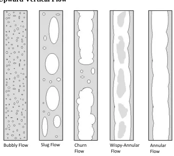
Figure 2: Flow regimes in vertical upward co-current gas/liquid flow

Although the current study deals with horizontal flow, vertical flow will be introduced as many of the flow patterns are subsequently found in a modified form in horizontal flow. Figure 2 details flow regimes as found in co-current vertical upward vapour/liquid flow. “Bubbly flow” usually occurs at low qualities and consists of small discrete bubbles dispersed within the liquid phase, the mean bubble diameter being much smaller than the channel diameter. As the quality increases, individual bubbles coalesce into slugs that almost fill the cross sectional of the channel or tube. This is usually referred to as “slug flow”. At higher vapour qualities, the vapour phase dominates the central area of the flow channel with the liquid remaining at the wall forming an annular flow film.

At intermediate qualities however, two additional regimes occur. For flows with high vapour and liquid flow rates, annular flow occurs, but with additional entrained “wisps”

Bubbly Flow Slug Flow Churn Flow

Wispy-Annular Flow

At intermediate quality, but with a lower liquid flow rate, an unstable region occurs where the imposed pressure gradient and gravity are similar in magnitude to the vapour shear on the liquid vapour interface. Although the mean velocity of the flow remains positive, the liquid experiences alternate positive and negative motion as gravity and liquid/vapour forces interact, thus producing an irregular interface. This is referred to as “churn flow”.

2.1.2:

Horizontal Flow

Figure 3 depicts the typical horizontal two-phase flow regimes. A similarity in pattern with vertical flow regimes is clear, except that the influence of gravity acts at 90° to the fluid flow. The denser liquid settles to the lower parts of the tube because of gravitational forces, while buoyancy causes the bubbles or slugs to migrate to the top of the tube.

As with vertical flow, “bubbly flow” is associated with lower qualities. In horizontal flow however the bubbles concentrate mainly along the top of the tube. With higher liquid velocity, shear forces may promote more even distribution of bubbles within the tube.

As the quality increases, coalescence leads to an increase in bubble size resulting in large oblong bullet shaped plugs, hence the title “plug flow”. These tend towards the top of the tube due to buoyancy forces.

With higher qualities combined with low flow rates, gravity and buoyancy provide a separation effect and “stratified flow” occurs where the liquid and vapour are separated by a smooth interface.

Figure 3: Flow regimes as observed in horizontal co-current gas liquid flow.

With higher liquid flow rates, the amplitude of the waves grows so large that the crests make contact with the upper surface of the tube or channel, forming a bridging effect. This forms large slugs similar to that found in vertical flow, and hence this is also known as “slug flow”.

2.1.3:

Single Phase Heat Transfer Correlations

Single phase heat transfer correlations can generally be divided into two areas, laminar flow and turbulent flow. In the fully developed laminar flow region of a tube flow, the expression for a constant heat flux has been shown to reduce to

36 . 4   k hD

Nu_D (12)

while for a constant wall temperature again this reduces to a constant

66 . 3   k hD

Nu_D (13)

For turbulent correlations, the calculations are more involved but again have been reduced to a form known as the Colburn equation

33 . 8 . Pr Re 023 . 0 _D D

Nu  (14)

This is then modified to become the more preferred Dittus-Boelter equation

n D D

Nu 0.023Re.8Pr (15)

where n=0.4 for heating and 0.3 for cooling. A further modification of the Dittus-Boelter equation to take account of property variations is the Sieder-Tate correlation

14 . 0 33 . 8 . Pr Re 027 . 0 _       s D D Nu   ₍₁₆₎

 

 

To accommodate smaller Reynolds numbers Gnielinski modified this form to become

 

 

All the correlations in this single phase subsection, as well as their range of validity and calculation details for the friction factor “f”, can be found in more detail in common heat transfer textbooks such as that of Bejan, Holman, and Incropera [15-17].

2.1.4:

Two Phase Flow Mapping

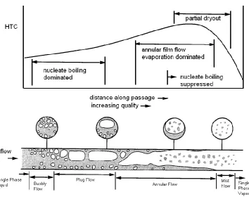
Figure 4: Variation of convective boiling heat transfer coefficient with flow regime, adapted from Kreith and Boehm [18]

According to Taitel [19], no less than 11 parameters can affect the flow pattern through a tube. These are shown in Table 1.

Table 1: Parameters which Influence Flow Pattern

Parameter Symbol Unit

1 Liquid superficial velocity jl m/s

2 Gas superficial velocity jv m/s

3 Liquid density ρL kg/m3

4 Gas density ρG kg/m3

5 Liquid viscosity μL kg/s m

6 Gas viscosity μG kg/s m

7 Pipe diameter D m

8 Acceleration due to gravity g m/s

9 Surface tension σ kg/s2

10 Pipe roughness ε m

Therefore, construction of heat transfer predictions must take into account, not only the parameters found in single-phase relations, such as geometric terms and dimensionless property characteristics like Reynolds and Prandtl numbers, but must also somehow account for the extra vapour properties, and include how the liquid and vapour are interacting. Hence studies revolve around precise determination of these flow regimes by varying flow rates, inlet quality and heat input. Thus flow regime mapping began as an aid to predict the flow regimes for given conditions where, once the flow regime was first determined, an applicable correlation could then be applied.

While certain elementary correlations have been put forward for two-phase flow, their derivation may not take account of the many flow regime factors discussed above. A more complete discussion of these correlations will be given in subsection 2.1.5: Two Phase Heat Transfer Correlations.

Figure 5: Vertical tube flow pattern map by Fair [20]

determines if the point is in the bubbly, slug, annular or mist flow regime. The Hewitt and Roberts map relates the superficial momentums of liquid and vapour phases. The flow regimes were determined by visual observation along a transparent tube, and the boundary lines between regimes demarcate the middle of a transition between those regimes.

Figure 6: Flow regime map proposed by Hewitt and Roberts [21]

The values of the x and y axes are then calculated to determine the flow regime. The Baker map is shown in Figure 7.

Figure 7: Baker flow map for horizontal tubes

From these flow maps, research focused on the delineation of the boundaries between flow regimes. Various analytical expressions for the transitions between these regimes have been obtained by various researchers and are now summarised.

In 1962, Radovcich and Moissis [22] proposed that bubble collision frequency could determine the transition from bubbly flow to slug flow at void fractions (α) greater than 0.3. Taitel and Dukler [23] later analysed this thesis further and proposed the relation









5 .

25 . 07

. 1 34 . 2

l v

v l

v l

j g j

j

 

 



buoyancy of the bubble slug, it moves upwards at a higher velocity than the two–phase flow average velocity, while the liquid actually moves downward. With further increases in quality and resultant void fraction, the plug bubble size increases and a Helmholtz type of instability arises precipitating the breakdown of the large plug bubbles and giving rise to churn flow. This transition was predicted to occur at conditions presented in a relation proposed by Porteus [24]









where D is the tube diameter. However Taitel and Dukler [23] argued that for

50 )

/( )

(j_l j_v gD 0.5 (23)

the slug to churn transition occurs when

16 . 0 / _v 

l j

j . (24)

The transition from churn flow to annular flow arises when the shear stress of the vapour core combined with the imposed pressure gradient balances the gravity force on the liquid film. Wallis [25] postulated that based on theoretical models, this occurred approximately when









5 . 0 . 2           _v l v v gD j    ₍₂₅₎

Taitel and Dukler [23] proposed a more involved correlation to predict the transition from churn to annular flow









 2 0.5

5 . 0 2 25 . 0 5 . 0 ) 20 1 ) 20 1 ( 09 . 3 X X X X X g j v l v v     ₍₂₆₎

5 . 0 ) / ) / (        v l dz dP dz dP X (27)

Here dP/dz is the frictional pressure gradient for the liquid and vapour phases as if they were flowing alone in the pipe, and methods of calculation are listed in Carey [14].

Taitel and Dukler developed the horizontal map shown in Figure 8, based on an analysis of flow transition mechanisms combined with empirical choice of specific parameters. The three part map uses the Martinelli parameter X, the gas Froude number FrG and the parameters T and K. The gas Froude number is defined as









i g l g g g g d ρ ρ ρ m Fr 

  (28)

Taitel and Dukler define T as the parameter









where g in both cases is the acceleration due to gravity =9.81 m/s2_. The parameter K is defined as

5 . 0 Re_l g Fr

K  (30)

The pressure gradient of the flow for phase k (where k is either l or g) is given by

i k k k k d m f dz dp  2 2 ) /

(   (31)

where fk , is the friction factor, which depends on the flow Reynolds number. If

k k

f

Re 16

 (32)

If Rek>2000, then the turbulent flow friction factor is used

25 . 0 Re

0079 . 0

k k

f  (33)

Figure 8: Taitel and Dukler Two-phase Flow Pattern Map, from [20]

Again, using T and X in the lower graph, the flow regime can be confirmed as either bubbly or intermittent flow. Although the Taitel and Dukler map is more complex to calculate, it does attempt to incorporate in the final calculation the flow characteristics found at various regimes.

Hashizume [26] in 1983 presented a flow map based on a modified form of the Baker map. This is shown in Figure 9. Hashizume found that the boundaries between the original Baker map and his modified map differed considerably due to the dissimilarity in surface tension properties of the refrigerant liquid and vapour from those of water and air as used by Baker.

Figure 9: Hashizume two-phase flow map[26]

Figure 10: Flow map form as proposed by Steiner

Figure 11: Flow map of Kattan, Thome and Favrat [28], sourced from [28]

The Kattan et al. map plots vapour quality on the x axis and mass velocity on the y, with curves and lines to delineate the boundaries between regimes. The Kattan et al. map places plug and slug flows in the Intermittent (I) classification, where the tube wall is assumed to remain constantly wetted due to the large waves which ensure a film of liquid on the top of the tube. Due to the axes being linear as in the Steiner map, interpretation is simpler than other log-log map formats. In addition, the Kattan et al. map avoids the use of iterative calculations by incorporating the Steiner modified version of the Rouhani-Axelsson drift flux model [30, 31] used to calculate the cross-sectional void fraction, ε. Complete equations for the curves defining the transitions between regimes can be found in the Wolverine Heat Transfer Engineering Data book III [20] and also in the publications of Kattan et al. [28-30].

Figure 12: Typical two-phase flow patterns dependent on mass flux and quality overlaid on a Kattan et al. type flow map [20]

The final flow map to be discussed is a follow-on from the Kattan et al. map. Wojtan, Ursenbacher and Thome [31] found that the flow regime during evaporation is highly influenced by nucleate boiling, evaporation of liquid, and acceleration of the flow as a result of this phase change. Consequently, Wojtan et al. revisited the map of Kattan et

al., using improved observation techniques, and proposed that the stratified wavy

Figure 13: Flow map of Wojtan, Ursenbacher and Thome, image from [31]

Another modification was made to the transition curve between stratified and stratified wavy below vapour qualities of xIA, where the intermittent to annular transition takes place, thus accuracy below Gwavy is improved.

2.1.5:

Two Phase Heat Transfer Correlations

Earlier methods of horizontal flow prediction in plain tubes were extensions of those derived from vertical upward flows. One of the earliest developed and widely used was the Chen correlation from 1966 [32]. Chen proposed a superpositional correlation for vertical channels that calculated the nucleate boiling contribution based on the Forster-Zuber pool boiling equation and then added the convective non-boiling contribution based on the Dittus Boelter equation (15). The final form is

F

S _L

FZ

tp  

75 . 0 24 . 0 24 . 0 24 . 0 29 . 0 5 . 0 49 . 0 45 . 0 79 . 0 00122 .

0 _{sat sat}

G LG L L pL L

FZ T p

h c k                 (35) and        i L D L d k 5 2 5 4 Pr Re 023 . 0  (36)

S is a nucleate boiling suppression factor, intended to take account of a steeper temperature gradient occurring in the liquid near the wall under forced convection conditions, which would lessen nucleation from that found in pool boiling. The other factor, F, is a two-phase multiplier which is used to augment the single phase contribution given by the Dittus-Boelter correlation. Details of both factors can be found in [20]. The difference between the inner tube wall and the liquid saturation temperature is ) T -(T

Tsat  wall sat

 (37)

Likewise the pressure difference, Δpsat is obtained from the vapour pressure of the fluid at that wall temperature, giving

) p -(p_{wall sat}

sat 

p (38)

This correlation is applicable for qualities 0.01<x<0.71 as long as the heated wall does not dry out. Iteration is necessary if the heat flux is specified as Twall and pwall are often not known.

Figure 14: Chart of Shah correlation, image from [33]

To use the chart, one first had to calculate the dimensionless parameters C0, the boiling number Bo and the Froude number FrL. For a vertical tube, the parameter C0 was then plotted on the x-axis and drawn vertically upward until it intersected the Bo line, whereupon a horizontal line was then drawn leftwards to intersect the y axis. Fr, being applicable to vertical tubes, was neglected. For horizontal tubes, a line was plotted from C0 as before but only to the intersection of the Fr number. Then a horizontal line was extended to the right to intersect the line A-B. From here another vertical line was extended to reach the Bo line and another horizontal line extended leftwards to read off the augmented heat transfer. Full details of the dimensionless parameters are given in Shah [33] and Collier [34].

The basic equation became

nb f

TP E S

   (39)

where αf was calculated using the Dittus-Boelter equation but using the local liquid fraction of the flow i.e., G(1-x). This convective component was then multiplied by the new convection enhancement factor E

       

 1.6 0.86

) 1 ( 37 . 1 000 . 24 1 tt X Bo E (40)

where Xtt is the Martinelli parameter as seen before, but in this case calculated as

1 . 0 5 . 0 9 . 0 5 . 0 1 ) / ) / (                                g f f g v l x x dz dP dz dP X     ₍₄₁₎

The nucleate boiling component was based on the reduced pressure correlation derived by Cooper [36]. This expression gives the heat transfer coefficient in W/m2_K.

67 . 0 5 . 0 55 . 0 12 . 0 ) ln 4343 . 0 (

55p_r p_r M q

nb      (42)

where M is the molecular weight, q is the heat flux in W/m2 _{and pr is the reduced} pressure which is the ratio of the saturation pressure psat to the critical pressure pcrit. Gungor and Winterton proposed an empirically derived boiling suppression factor S





Re 00000115 .

0

1 

 E f

S (43)

with Ref alsobased on G(1-x).

In 1992, Steiner and Taborek [20, 34, 37] provided a mechanistic model which would take into account the principles of pool and convective boiling terms. They proposed combining both convective and nucleate boiling contributions using a power law of the form





C n nb tp h h

h

1

) ( )

( 

 (44)

Steiner and Taborek proposed that the following limits should apply to evaporation in vertical tubes: For heat fluxes below the threshold for the onset of nucleate boiling (q’’

< q’’ONB ), the nucleate boiling contribution should not be included, only the convective

contribution.

For very large heat fluxes, the dominative term should be nucleate boiling.

When the inlet quality is zero, the two-phase heat transfer coefficient, htp, should equal the single-phase liquid convective heat transfer coefficient when heat flux is less than the heat flux for the onset of nucleate boiling (q’’ <q’’ONB), but, htp should correspond to that plus hnb when q’’ > q’’ONB .

When x = 1.0, htp should equal the vapour-phase convective coefficient (the forced

Figure 15: Steiner-Taborek description of boiling processes in a vertical tube

The Steiner-Taborek depiction of flow boiling in a vertical tube is shown in Figure 15 and the regions A-G are described in the following text.

Region A-B

q>qONB. During subcooled boiling, the growth and collapse of bubbles near the wall increases heat transfer.

Region B-C_D

Only convective evaporation occurs when q<qONB, as indicated by the “pure convective boiling” curve. Both nucleate and convective boiling contributions are present and can be superimposed when q>qONB. The nucleate boiling coefficient at the particular heat flux is shown by horizontal dashed lines while the solid curves are the superimposed contribution of nucleate and convective boiling that together constitute htp. The flow pattern as shown in the bottom diagram transits through both bubbly flow and churn flow regimes.

Region D-E-F

When q<qONB, the process continues along the pure convective boiling curve up to the onset of dryout at high vapour qualities approaching x=1.0. The annular flow regime constituting a thin turbulent annular liquid layer on the tube wall and a central vapour core, is reached when q>qONB, and continues up to the point where the critical vapour quality xcrit is reached, after which the annular film dries out.

Region F-G

The liquid film at xcrit is subject to instability from interfacial shear and adhesion forces. The heat transfer mechanisms also change in the mist flow regime, where heat transfer is now by vapour-phase convection, by evaporation of entrained liquid droplets within the superheated vapour, by droplets impinging onto the tube wall, and by radiation.

Based on the power-law type equation (62), Steiner and Taborek now proposed the correlation





1 3 3

, ) ( )

( _{nbo nb Lt tp}

tp h F h F

h   (45)

Fnb is the nucleate boiling correction factor (not a suppression factor, as this is an asymptotic model)

hLt is the local liquid-phase forced convection coefficient based on the total flow as liquid (as opposed to liquid fraction of flow shown in earlier methods) derived from the Gnielinski correlation instead of the Dittus-Boelter correlation.

Ftp is the phase multiplier accounting for the higher velocity of liquid in a two-phase flow – a flow regime which gives higher heat transfer enhancement as opposed to a lower-velocity single-phase flow.

A more complete description of the Steiner-Taborek model including full details of the terms relating to equation (63) is provided in Collier and Thome [34].

While the correlations of Chen [32], Shah [33], Gungor and Winterton [38] were vertical flow correlations, modifications of these models were developed in order to fit flow in horizontal tubes. One simple modification was made by Shah to his vertical tube correlation presented earlier, where he set a threshold delineating stratified and non-stratified flow based on the liquid Froude number. Below the threshold FrL=0.4, the normal vertical correlation is applied. Above that threshold, a modified N term is introduced to take account of the stratification. Gungor and Winterton also utilised the liquid Froude number based threshold, but set the value of FrL=0.05, and in addition modified both their convective enhancement and boiling suppression (E and S) terms.

However, while the methods offer simple calculation and perform well in the annular flow regime, certain limitations were noted [20] when these correlations are used for other flow regimes;

They only predict stratified and non-stratified flows and accommodate neither other flow regimes nor the transition from unstratified to stratified flow.

Plotting the predicted HTC values versus quality (x) often do not reflect actual experimental values or trends.

They do not take into account the region near dryout. They hence can both under-predict heat transfer before this region and over-under-predict heat transfer after the onset of dryout - in some cases by up to 300%.

Consequently, a more phenomenological approach proposed by Kattan, Thome and Favrat [28-30] was developed related to their flow map described earlier. Cotton [4], reviewing various two-phase correlations, also favours this approach over previous methods as it includes mechanisms to account for the effects of local two-phase flow patterns, flow stratification and partial dryout. This phenomenological study was greatly facilitated by use of visualisation tools such as high-speed cameras and laser equipment in order to properly define flow regimes and their boundaries. Optical methods were also utilised by Kattan et al. to measure liquid/vapour transitions passing a particular point of the tube, and this was then related to void fraction and used in their calculations of flow regimes.

The Kattan, Thome and Favrat map represents simplified two-phase flow structures of fully stratified, stratified-wavy, and annular flow regimes, based on the flow map seen in Figure 11. The simplified structures are shown in Figure 16. The two upper drawings depict stratified flow, while the lower three show the transition from annular to stratified flow.

Figure 16: Simplified flow structures proposed in Kattan Thome Favrat Model, adapted from [20, 30]

and the subsequent flow regime calculations are detailed by Kattan et al. in [28-30]. The general equation for the flow boiling coefficient in a horizontal tube is given by





The dry perimeter of the tube is given by the dry angle θdry and the corresponding heat transfer is given by αvapour. αwet denotes the heat transfer coefficient on the wetted perimeter and this is made up of an asymptotic expression combining nucleate boiling and convective boiling and using an exponent of three giving:





1 3 3

cb nb

wet  

   (47)

A reduced pressure correlation, put forward by Cooper and used to determine αnb , is





12 . 0

log

55p_r p_r M q

nb 



 



M is the liquid molar weight, pr is the reduced pressure, and q is the heat flux at the wall in W/m2_{K. The convective boiling heat transfer coefficient of the annular film of} liquid is given by

      L L L pL L cb k k c x

m 0.69 0.4

) 1 ( ) 1 ( 4 0133 . 0 _             

  (49)

The first term in brackets is the liquid Reynolds number calculated on the mean velocity of the liquid which is a function of t