An Iteration Method using Elliptical Arc Artificial Boundary for Exterior Problems

An Iteration Method using Elliptical Arc Artificial

Boundary for Exterior Problems

Yajun Chen, and Qikui Du

Abstract—In this paper, an iteration method using elliptical arc artificial boundary is designed to solve exterior Poisson problem with a concave angle. It is shown that the iteration method is equivalent to a Schwarz alternating method. The convergence of this method is given. The convergence rate is analyzed in details for a typical domain. Finally, some numerical examples are given, which show the effectiveness of the iteration method.

Index Terms—Schwarz alternating method, elliptical arc artificial boundary, exterior problem.

I. INTRODUCTION

T

HE problems in unbounded media are encountered in a variety of applications. To solve such problems in infinite region numerically, there is a variety of numerical methods. One commonly method is the method of artificial boundary conditions [1]-[7]. The method may be summa-rized as follows: (i) Introduce an artificial boundary Γµ, which divides the original unbounded domain into two non-overlapping subdomains: a bounded computational domain

Ωi and infinite residual domain Ωe. (ii) By analyzing the problem inΩe, obtain a relation onΓµ(exact or approximate) involving the unknown function u and its derivatives. (iii) Using the relation as a boundary condition on Γµ, to obtain a well-posed problem inΩi. (iv) Solve the problem inΩi be the standard finite element methods or some other numerical methods. The relation obtained in Step (ii) and used as a boundary condition in Step (iii) is called an artificial boundary condition.

In the past three decades, artificial boundaries of various shapes have been derived for problems in unbounded do-mains [8]-[18]. Recently, the authors used a new elliptical arc artificial boundary to solve Poisson problems and anisotropic problems in concave angle domains [19]-[20]. In this paper, we design an iteration method to solve exterior Poisson problem with a concave angle. Using the results of [19]-[20] with an artificial boundary we change the original problem to an equivalent problem in a bounded domain. Then an iteration method is designed to solve the new problem. The convergence of the iteration is obtained by showing that the iteration is actually equivalent to the standard Schwarz alternating method.

LetΩbe an exterior concave angle domain with angleα, and0< α≤2π. The boundary of domainΩis decomposed into three disjoint parts:Γ,Γ0andΓα(see Fig. 1), i.e.∂Ω =

Manuscript received December 29, 2016; revised February 22, 2017. This work was supported by the National Natural Science Foundation of China (Grant No. 11371198).

Yajun Chen is with the School of Mathematical Sciences, Nanjing Normal University, Nanjing 210023 and the Department of Mathematics, Shanghai Maritime University, Shanghai 200136, China (E-mail: [email protected]).

Qikui Du is with the School of Mathematical Sciences, Nanjing Normal University, Nanjing 210023, China.

α

Γ

Γ

0

Γ

α

[image:1.595.312.483.355.500.2]

Ω

Fig. 1. The Illustration of DomainΩ

Γ∪Γ0∪Γα,Γ0∩Γα= Ø,Γ∩Γ0= Ø,Γ∩Γα= Ø. The boundary Γ is a simple smooth curve part, Γ0 and Γα are two half lines.

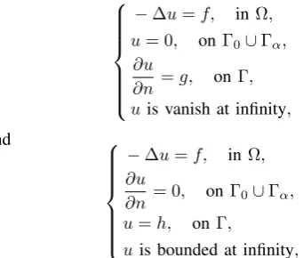
We consider the Poisson problem in two cases: 

           

−∆u=f, inΩ, u= 0, onΓ0∪Γα,

∂u

∂n =g, onΓ, uis vanish at infinity,

(1)

and 

           

−∆u=f, inΩ, ∂u

∂n = 0, on Γ0∪Γα, u=h, onΓ,

uis bounded at infinity,

(2)

where u is the unknown function, f ∈ L2_{(Ω) and g, h ∈} L2_{(Γ)are given functions, supp(f) is compact.}

The rest of the paper is organized as follows. In Section 2, we introduce two elliptical arc artificial boundaries which divide the original domain Ω into two subdomains, then we construct an iteration method which is equivalent to a Schwarz alternating method. In Section 3, we give the convergence of the method . In Section 4, we analyze the convergence rate for a typical domain. In Section 5, we give the discretization of the method. Finally, in Section 6 we present some numerical results, check its accuracy and the effectiveness of this method.

II. ITERATION BASED ON THE ELLIPTICAL ARC ARTIFICIAL BOUNDARY CONDITION

We introduce two elliptical arc artificial boundariesΓ1and Γ2 with the same foci, Γi = {(µ, φ)|µ = µi,0 < φ <

α}, i= 1,2, which encloseΓ such that dist(Γ,Γ2)>0 and µ1 > µ2 >0. Here(µ, φ)denotes the elliptic coordinates,

x=f0coshµcosφ,y =f0sinhµsinφ. ThenΩis divided into two overlapping subdomainsΩ1andΩ2(see Fig. 2). Let Ω1be the bounded domain amongΓ,Γ0,ΓαandΓ1, andΩ2

be the unbounded domain outsideΓ2,Γ0 andΓα. Then the

IAENG International Journal of Applied Mathematics, 47:2, IJAM_47_2_10

[image:2.595.307.547.418.592.2]

α

Γ

Γ

1

Γ

0

Γ

α

Ω

1

Ω

2

Γ

2

Fig. 2. The Illustration of DomainΩ1 andΩ2

original problem (1) is decomposed into two subproblems in domains Ω1 and Ω2 withΩ1∩Ω2 ̸= Ø,∂Ω1 = Γ∪Γ1∪ Γ01∪Γα1,∂Ω2 = Γ2∪Γ02∪Γα2. where Γ0i = Ωi∩Γ0, Γαi= Ωi∩Γα,i= 1,2. Assume thatf = 0in the domain

Ω2.

In the first case, we consider the following problem:

        

−∆u= 0, inΩ2, u= 0, on Γ02∪Γα2,

u=uµ2, on Γ2,

uis vanish at infinity.

(3)

It is well-known that the solution of this problem has the form

u(µ, φ) = +_∞

∑

n=1

bne(µ2−µ)

nπ

α sinnπφ

α . (4)

From (4) we obtain the coefficientsbn,n= 1,2, . . .

bn =

2 α

∫ α

0

uµ2(µ2, ϕ) sin

nπϕ α dϕ.

Thus (4) can be written as

u(µ, φ)

= 2 α

+∞

∑

n=1

e(µ2−µ)nπα _sinnπφ α

∫ α

0

uµ2(µ2, ϕ) sin

nπϕ α dϕ

≡H(uµ2, µ, φ).

(5)

Using expression (5) we can construct an iteration method for problems (1). From (5) the solutionuof (1) restricted on

Γ1can be expressed as

u(µ1, φ) =H(uµ2, µ1, φ).

Then in the domain Ω1 problems (1) is equivalent to the

following problem:             

−∆u=f, inΩ1, u= 0, on Γ01∪Γα1,

∂u

∂n=g, on Γ, u=H(uµ2, µ1, φ).

Since uµ2 is unknown, we construct the following iteration

method to solve this problem:               

−∆u(2₁k+1)=f, inΩ1, u(2₁k+1)= 0, onΓ01∪Γα1,

∂u1 ∂n

(2k+1)

=g, on Γ,

u₁(2k+1)=H(uµ(22k), µ1, φ), onΓ1,

(6)

whereu(2µ2k)=u

(2k)_(µ 2, φ).

It is not difficult to see that the above iteration method is actually equivalent to the following Schwarz alternating method:               

−∆u(2₁k+1)=f, inΩ1, u(2₁k+1)= 0, onΓ01∪Γα1,

∂u1 ∂n

(2k+1)

=g, onΓ,

u(2₁k+1)=u₂(2k), onΓ1, k= 0,1, . . .

(7) and             

−∆u(2₂k+2)=f, inΩ2, u(2₂k+2)= 0, onΓ02∪Γα2,

u(2₂k+2)=u(2₁k+1), onΓ2,

u(2₂k+2)is vanish at infinity, k= 0,1, . . .

(8)

For the second case, we can also construct the following Schwarz alternating method:

              

−∆u(2₁k+1)=f, inΩ1, ∂u1

∂n (2k+1)

= 0, onΓ01∪Γα1,

u(2₁k+1)=h, onΓ,

u(2₁k+1)=u₂(2k), onΓ1, k= 0,1, . . .

(9) and               

−∆u(2₂k+2)=f, inΩ2, ∂u2

∂n (2k+2)

= 0, on Γ02∪Γα2,

u(2₂k+2)=u(2₁k+1), onΓ2,

u(2₂k+2) is bounded at infinity, k= 0,1, . . .

(10)

Taking some initial value of function u0 on boundary Γ1, e.g. u|Γ1 = 0. Combining it with the given boundary condition onΓ01∪Γα1∪Γ, we can solve the interior boundary

value problem in domainΩ1, get the value of solutionu1|Γ2 onΓ2, and then solve the exterior boundary value problem

in domain Ω2, get the value of solution u2|Γ1 on Γ1, and then solve the problem inΩ1 again, ..., and so on.

In the following sections, we just consider the convergence and convergence rate of problem (1), we can obtain corre-sponding result of problem (2) in the same way.

III. CONVERGENCE OF THE METHOD

The solution of problems (1) is in space

V ={v∈W01(Ω)|v= 0, on Γ0∪Γα},

IAENG International Journal of Applied Mathematics, 47:2, IJAM_47_2_10

where

W₀1(Ω)

={v|√ v

x2_+y2_{+ 1 ln(x}2_+y2_{+ 2)}, ∂v ∂x,

∂v ∂y ∈L

2_(Ω)}.

Functions u(2₁k+1) ∈ H(Ω1) and u (2k)

2 ∈ W01(Ω2) can be

extended to functions in V. Let

V1={v∈H1(Ω1)|v= 0, on Γ01∪Γα1∪Γ1},

V2={v∈W₀1(Ω2)|v= 0, onΓ02∪Γα2∪Γ2}.

Then

u(2₁k+1)−u(2₂k)∈V1, u(2₂k+2)−u(2₁k+1)∈V2.

We can look uponV1andV2as the subspaces ofV. Define the bilinear form as follows

a(u, v) = ∫

Ω

∇u∇vdx.

From this, the inner producta(u, v)and the norm∥v∥1inV

can be defined. Then (7) and (8) are equivalent to variational problems

{

Find u(2₁k+1)∈V1+u (2k)

2 , such that a(u(2₁k+1)−u, v1) = 0, ∀v1∈V1,

(11)

and {

Find u(2₂k+2)∈V2+u(2₁k+1), such that

a(u(2₂k+2)−u, v2) = 0, ∀v2∈V2.

(12)

LetPVi :V →Vi,i= 1,2 denote the orthogonal projectors

under the inner product a(·,·). We have {

u₁(2k+1)−u₂(2k)=PV1(u−u

(2k) 2 ), u₂(2k+2)−u₁(2k+1)=PV2(u−u

(2k+1)

1 ), k= 0,1, . . . ,

(13) or equivalently

{

u−u(2₁k+1)=P_V⊥

1 (u−u

(2k) 2 ), u−u(2₂k+2)=P_V⊥

2 (u−u

(2k+1)

1 ), k= 0,1, . . .

(14)

whereV_i⊥,i= 1,2are the orthogonal complementary spaces of Vi inV. Let

{

e₁(2k+1)=u−u₁(2k+1), k= 0,1, . . . , e₂(2k)=u−u₂(2k), k= 1,2, . . .

be errors. Then (14) is {

e(2₁k+1)=PV₁⊥e

(2k)

2 , k= 1,2, . . . , e(2₂k+2)=PV₂⊥e

(2k+1)

1 , k= 0,1, . . .

Therefore {

e(2₁k+1)=P_V⊥

1 PV2⊥e

(2k−1)

1 , k= 1,2, . . . , e(2₂k+2)=P_V⊥

2 PV1⊥e

(2k)

2 , k= 0,1, . . .

This implies that, if {e(2₁k+1)} and {e(2₂k)} are convergent, then their limits are inV₁⊥∩V₂⊥. Similar to the proofs given in [21]-[22] we can show the following results

Theorem 1. lim

k→∞∥e

(2k+1)

1 ∥1= 0, lim

k→∞∥e

(2k) 2 ∥1= 0.

Theorem 2. There exists a constantδ,0 6 δ < 1, such that

∥e(2₁k+1)∥16δk∥e (1)

1 ∥1, ∥e (2k)

2 ∥16δk∥e (0) 2 ∥1.

Theorems 1 and 2 show that the Schwarz alternating method converges geometrically, and the contraction factor is δ. We find it is quite difficult to analyze the rate of convergence δ for general unbounded domain Ω. However, it is possible to findδwhen Γis an elliptical arc, it will be given in next section.

IV. ANALYSIS OF CONVERGENCE RATE

For simplicity, we letΓ,Γ1andΓ2 be elliptical arcs with

the same foci, Γ = {(µ, φ)|µ = µ0,0 < φ < α}, Γi = {(µ, φ)|µ =µi,0 < φ < α}, i= 1,2, and µ1 > µ2 > µ0.

Let

e(0)₂ (µ1, φ) = +∞

∑

n=1 bnsin

nπφ

α (15)

is given on the artificial boundaryΓ1and

∂e(1)₁

∂µ = 0, onΓ. (16)

And let

e(1)₁ (µ, φ) = +∞

∑

n=1 (Ane

nπµ

α _+Bne− nπµ

α _{) sin}nπφ

α , inΩ1.

From (15) and (16) we have

An=

bne−

nπµ₀ α

enπα(µ1−µ0)+enπα(µ0−µ1) ,

Bn=

bne

nπµ0

α

enπα(µ1−µ0)_+enπα(µ0−µ1). Hence

e(1)₁ (µ, φ) = +_∞

∑

n=1

enπα(µ−µ0)_+enπα(µ0−µ)

enπα(µ1−µ0)_+enπα(µ0−µ1)bnsin

nπφ α .

Therefore

e(1)₁ (µ2, φ) = +∞

∑

n=1

enπα(µ2−µ0)_+enπα(µ0−µ2)

enπα(µ1−µ0)+enπα(µ0−µ1) bnsin

nπφ α .

Using (4), we can obtain the value of function onΓ1

e(2)₂ (µ1, φ)

= +∞

∑

n=1

enπα(µ2−µ1)e

nπ

α(µ2−µ0)_+enπα(µ0−µ2)

enπα(µ1−µ0)+enπα(µ0−µ1) bnsin

nπφ α .

So

∥e(2)₂ ∥21 2,Γ1

= +∞

∑

n=1

(1 +n2)12|_enπα(µ2−µ1)e nπ

α(µ2−µ0)_+enπα(µ0−µ2)

enπα(µ1−µ0)_+enπα(µ0−µ1)bn|

2

6 +∞

∑

n=1

(1 +n2)12|_enπα(µ2−µ1)_bn|2

6e2απ(µ2−µ1) +_∞

∑

n=1

(1 +n2)12|_bn|2

=e2απ(µ2−µ1)∥_e(0) 2 ∥

2

1 2,Γ1.

IAENG International Journal of Applied Mathematics, 47:2, IJAM_47_2_10

Similarly, we can obtain

∥e(3)₁ ∥21 2,Γ26e

2π

α(µ2−µ1)∥e(1) 1 ∥

2

1 2,Γ2. Using mathematics induction, we have

∥e(2₂k)∥21 2,Γ1 6e

2kπ

α (µ2−µ1)∥_e(0)

2 ∥ 2

1

2,Γ1, k= 1,2, . . . , ∥e(2₁k+1)∥21

2,Γ2 6e 2kπ

α (µ2−µ1)∥_e(1)

1 ∥ 2

1

2,Γ2, k= 1,2, . . . Therefore, we have

Theorem 3. Let Γ, Γ1 and Γ2 be elliptical arcs with

the same foci, Γ = {(µ, φ)|µ = µ0,0 < φ < α},

Γi = {(µ, φ)|µ = µi,0 < φ < α}, i = 1,2, and

µ1> µ2> µ0. If we apply the Schwarz alternating method

given in Section 2 to problem (1), then

∥e(2₂k)∥1 2,Γ1 6δ

k_∥e(0) 2 ∥1

2,Γ1, k= 1,2, . . . , ∥e(2₁k+1)∥1

2,Γ2 6δ k_∥e(1)

1 ∥1

2,Γ2, k= 1,2, . . . , whereδ=eπα(µ2−µ1).

Finally, using the trace theorem we have

∥e(2₂k)∥1,Ω2 6Cδ k

, k= 1,2, . . . ,

∥e(2₁k+1)∥1,Ω16Cδ

k_{, k= 1,2, . . .}

The smaller theµ2−µ1 is, the faster the convergence is.

V. DISCRETIZATION

The bounded domain Ω1 is divided into triangular finite

element subdivisions. The subdivisions of Γ0, Γα, Γ1 and Γ2areΓ0h,Γαh,Γ1handΓ2h, respectively. The subdivision of elliptical arc Γ2 is Γ2φ. Let Sh(Ω1h), Sh(Γ1h) and

Sh_(Γ

2φ)are finite element function spaces, respectively, in

Ω1h, onΓ1h andΓ2h. Then we can obtain discrete Schwarz

alternating algorithm as follows:

Step 0. Put any initial datau0

φ∈C(Γ1),k:= 0.

Step 1. Findu(2_1hk+1)∈Sh_(Ω

1h), such that 

     

ah(u

(2k+1)

1h , vh) =fh(vh), vh∈S h_(Ω

1h),

u(2_1hk+1)= 0, onΓ01∪Γα1, u(2₁k+1)= Πhu

(2k)

2φ , onΓ1h.

(17)

Step 2. Findu(2_2φk+2)∈Sh_(Γ

2φ), such that 

           

−∆u(2_2φk+2)= 0, inΩ2, u(2_2φk+2)= 0, onΓ02∪Γα2,

u(2_2φk+2)= Πφu

(2k+1)

1h , onΓ2φ,

u(2_2φk+2)is vanish at infinity.

(18)

Step 3.

εk = max{ max

node∈Γ1h

|u(2_1hk+1)−u(2_1hk−1)|,

max

node∈Γ2φ

|u(2_2φk+2)−u(2_2φk)|}.

Step 4. Ifεk is small, stop; else goto Step 1.

where ah(u, v) = ∫

Ω1h∇u∇vdx, fh(v) =

∫

Ω1hf vdx+

∫

Γhgvds, Πh : C(Γ1) → S

h_(Γ

[image:4.595.339.511.57.144.2]

1h) is the interpolation operator, Πφ : C(Γ2) → Sh(Γ2φ) is the interpolation operator, too. Here Step 1 is solved by finite element method inΩ1h. Step 2 can be solved by artificial boundary condition.

Fig. 3. Meshhof SubdomainΩ1for Example 1

TABLE I

THERELATIONBETWEENCONVERGENCERATE ANDMESH FOR

EXAMPLE1 (µ1= 3,µ2= 2)

Mesh k 1 2 3 4 5

e(k) 0.1182 0.0878 0.0746 0.0688 0.0664

h/2 eh(k) 0.1133 0.0491 0.0213 0.0093 0.0040

qh(k) 2.3049 2.3045 2.3044 2.3044

e(k) 0.1018 0.0483 0.0294 0.0227 0.0198

h/4 eh(k) 0.1214 0.0535 0.0236 0.0104 0.0046

qh(k) 2.2685 2.2685 2.2685 2.2685

e(k) 0.0996 0.0450 0.0208 0.0101 0.0069

h/8 eh(k) 0.1235 0.0547 0.0242 0.0107 0.0047

qh(k) 2.2593 2.2593 2.2593 2.2592

VI. NUMERICAL EXAMPLES

In this section, we give two numerical examples to show the effectiveness of the Schwarz alternating method. In these examples, the exact solutions are known. The purpose of showing these examples is to check the convergence in terms of iteration k and mesh size h. The finite element method with liner elements is used in the computation. u1h is the finite element solution in Ω1,e andeh denote the maximal error of all node functions inΩ1, respectively, i.e.,

e(k) = sup

P_i∈Ω1

|u(Pi)−u12hk+1(Pi)|,

eh(k) = sup Pi∈Ω1

|u2₁k_h−1(Pi)−u21kh+1(Pi)|.

qh(k)is the approximation of the convergence rate, i.e.,

qh(k) =

eh(k−1)

eh(k)

.

Example 1. We consider problem (1), where Ω =

{(µ, φ)|µ > 1,0 < φ < 2π}, Γ = {(1, φ)|0 < φ < 2π},

Γ0 ={(µ,0)|µ > 1}, Γα ={(µ,2π)|µ > 1} and f0 = 2. Letu(µ, φ) = sin

φ

2

coshµ₂+sinhµ₂ be the exact solution of original

problem and g = ∂u_∂n|Γ. LetΓµi ={(µi, φ)|0 < φ < 2π}, i= 1,2 be the artificial boundaries. Fig. 3 shows the mesh

h of subdomain Ω1, Table 1 shows the relation between

convergence rate and mesh (µ1 = 3, µ2 = 2), Table 2 shows the relation between convergence rate and overlapping degree (mesh h/4, µ1 = 3), Fig. 4 shows L∞(Ω1) errors

with iterationk.

Example 2. We consider problem (1), where Ω =

{(µ, φ)|µ > 1,0 < φ < 3₂π}, Γ = {(1, φ)|0 < φ < 3₂π},

Γ0 = {(µ,0)|µ > 1}, Γα = {(µ,3₂π)|µ > 1} andf0 = 2. Let u(µ, φ) = sin

2φ

3

cosh2₃µ+sinh2₃µ be the exact solution of

original problem andg= ∂u_∂n|Γ. LetΓµi ={(µi, φ)|0< φ < 2π},i = 1,2 be the artificial boundaries. Fig. 5 shows the

IAENG International Journal of Applied Mathematics, 47:2, IJAM_47_2_10

TABLE II

THERELATIONBETWEENCONVERGENCERATE ANDOVERLAPPING

DEGREE FOREXAMPLE1 (MESHh/4,µ1= 3)

µ2 k 1 2 3 4 5

e(k) 0.0740 0.0310 0.0217 0.0187 0.0178 1.5 eh(k) 0.1492 0.0467 0.0146 0.0046 0.0014

qh(k) 3.1953 3.1942 3.1949 3.1949

e(k) 0.1018 0.0483 0.0294 0.0227 0.0198 2 eh(k) 0.1214 0.0535 0.0236 0.0104 0.0046

qh(k) 2.2685 2.2685 2.2685 2.2685

e(k) 0.1476 0.0984 0.0663 0.0454 0.0339 2.5 eh(k) 0.0755 0.0492 0.0321 0.0209 0.0136

qh(k) 1.5344 1.5343 1.5342 1.5342

0 5 10 15 20

10−3 10−2 10−1 100

Error

Iteration k

[image:5.595.312.539.87.354.2]

h/2 h/4 h/8

[image:5.595.58.283.87.357.2]

Fig. 4. L∞(Ω1)Errors with Iterationkfor Example 1

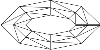
Fig. 5. Meshhof SubdomainΩ1for Example 2

TABLE III

THERELATIONBETWEENCONVERGENCERATE ANDMESH FOR

EXAMPLE2 (µ1= 3,µ2= 2)

Mesh k 1 2 3 4 5

e(k) 0.0794 0.0682 0.0648 0.0638 0.0635

h/2 eh(k) 0.0824 0.0250 0.0076 0.0023 0.0007

qh(k) 3.2922 3.2922 3.2922 3.2922

e(k) 0.0450 0.0233 0.0192 0.0180 0.0176

h/4 eh(k) 0.0903 0.0279 0.0086 0.0027 0.0008

qh(k) 3.2321 3.2321 3.2321 3.2321

e(k) 0.0429 0.0141 0.0064 0.0051 0.0047

h/8 eh(k) 0.0925 0.0287 0.0089 0.0028 0.0009

qh(k) 3.2162 3.2162 3.2162 3.2162

meshhof subdomainΩ1, Table 3 shows the relation between

convergence rate and mesh (µ1= 3,µ2= 2), Table 4 shows the relation between convergence rate and overlapping degree (mesh h/4, µ1 = 3), Fig. 6 shows L∞(Ω1) errors with

iterationk.

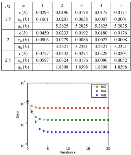
The numerical results show that this method is feasible and convergent quickly. Its convergence rate is related to the degree of overlapping of subdomains. The higher the

TABLE IV

THERELATIONBETWEENCONVERGENCERATE ANDOVERLAPPING

DEGREE FOREXAMPLE2 (MESHh/4,µ1= 3)

µ2 k 1 2 3 4 5

e(k) 0.0293 0.0196 0.0178 0.0175 0.0174 1.5 eh(k) 0.1061 0.0201 0.0038 0.0007 0.0001

qh(k) 5.2825 5.2825 5.2825 5.2825

e(k) 0.0450 0.0233 0.0192 0.0180 0.0176 2 eh(k) 0.0903 0.0279 0.0086 0.0027 0.0008

qh(k) 3.2321 3.2321 3.2321 3.2321

e(k) 0.0757 0.0432 0.0274 0.0228 0.0204 2.5 eh(k) 0.0597 0.0324 0.0176 0.0096 0.0052

qh(k) 1.8398 1.8398 1.8398 1.8398

0 5 10 15 20

10−3 10−2 10−1 100

Iteration k

Error

h/2 h/4 h/8

Fig. 6. L∞(Ω1)Errors with Iterationkfor Example 2

overlapping degree of the two subdomains is, the faster the convergence is. Moreover, the convergence rate is nearly not affected by finite element mesh.

ACKNOWLEDGMENT

The authors would like to thank the reviewers for their valuable comments which improve the paper.

REFERENCES

[1] H. Han, and X. Wu, “Approximation of infinite boundary condition and its application to finite element methods,”Journal of Computational Mathematics, vol. 3, no. 2, pp. 179-192, 1985.

[2] H. Han, and X. Wu,The artificial boundary method – numerical solu-tions of partial differential equasolu-tions on unbounded domains. Tsinghua University Press, Beijing, 2009.

[3] K. Feng, “Finite element method and natural boundary reduction,” in

Proceedings of International Congress Mathematicians, 1983, Warsza-wa, pp. 1439-1453.

[4] K. Feng, and D. Yu, “Canonical integral equations of elliptic boundary value problems and their numerical solutions,” inProceedings of China-France Symposium on the Finite Element Methods, 1983, Beijing, pp. 211-252.

[5] D. Yu,Natural Boundary Integral Method and Its Applications. Kluwer Academic Publishers, Massachusetts, 2002.

[6] J. B. Keller, and D. Givoli, “Exact non-reflecting boundary conditions,”

Journal of Computational Physics, vol. 82, no. 1, pp. 172-192, 1989. [7] M. J. Grote, and J. B. Keller, “On non-reflecting boundary conditions,”

Journal of Computational Physics, vol. 122, no. 2, pp. 231-243, 1995. [8] D. Yu, “Approximation of boundary conditions at infinity for a harmonic equation,”Journal of Computational Mathematics, vol. 3, no. 3, pp. 219-227, 1985.

[9] H. Han, and W. Bao, “Error estimates for the finite element approxima-tion of problems in unbounded domains,”SIAM Journal on Numerical Analysis, vol. 37, no. 4, pp. 1101-1119, 2000.

[10] H. Han, C. He, and X. Wu, “Analysis of artificial boundary conditions for exterior boundary value problems in three dimensions,”Numerische Mathematik, vol. 85, no. 3, pp. 367-386, 2000.

[11] G. Ben-Poart, and D. Givoli, “Solution of unbounded domain prob-lems using elliptic artificial boundaries,”Communications in Numerical Methods in Engineering, vol. 11, no. 9, pp. 735-741, 1995.

IAENG International Journal of Applied Mathematics, 47:2, IJAM_47_2_10

[image:5.595.84.255.391.476.2]

[12] D. Yu, and Z. Jia, “Natural integral operator on elliptic boundaries and a coupling method for an anisotropic problem,”Mathematica Numerica Sinica, vol. 24, no. 3, pp. 375-384, 2002.

[13] Q. Zheng, J. Wang, and J. Li, “The coupling method with the Natural Boundary Reduction on an ellipse for exterior anisotropic problems,”

Computer Modeling in Engineering and Sciences, vol. 72, no. 2, pp. 103-113, 2011.

[14] H. Huang, D. Liu, and D. Yu, “Solution of exterior problem using ellipsoidal artificial boundary,”Journal of Computational and Applied Mathematics, vol. 231, no. 1, pp. 434-446, 2009.

[15] D. Yu, “Coupling canonical boundary element method with FEM to solve harmonic problem over cracked domain,”Journal of Computa-tional Mathematics, vol. 1, no. 3, pp. 195-202, 1983.

[16] M. Yang, and Q. Du, “A Schwarz alternating algorithm for elliptic boundary value problems in an infinite domain with a concave angle,”

Applied Mathematics and Computation, vol. 159, no. 1, pp. 199-220, 2004.

[17] B. Liu, and Q. Du, “The coupling of NBEM and FEM for quasilinear problems in a bounded or unbounded domain with a cocave angle,”

Journal of Computational Mathematics, vol. 31, no. 3, pp. 308-325, 2013.

[18] Z. Dai, Q. Du, and B. Liu, “Schwarz alternating methods for anisotrop-ic problems with prolate spheroid boundaries,”SpringerPlus, vol. 5, pp. 1423-1423, 2016.

[19] Y. Chen, and Q. Du, “Solution of exterior problems using elliptical arc artificial boundary,”Engineering Letters, vol. 24, no. 2, pp. 202-206, 2016.

[20] Y. Chen, and Q. Du, “Artificial boundary method for anisotropic problems in an unbounded domain with a concave angle,” IAENG International Journal of Applied Mathematics, vol. 46, no. 4, pp. 600-605, 2016.

[21] D. Yu, “A domain decomposition method based on the natural bound-ary reduction over an unbounded domain,” Mathematica Numerica Sinica, vol. 16, no. 4, pp. 448-459, 1994.

[22] X. Wu, and C. Cheung, “An iteration method using artificial boundary for some elliptic boundary value problems with singularities,” Interna-tional Journal for Numerical Methods in Engineering, vol. 46, no. 11, pp. 1917-1931, 1999.

IAENG International Journal of Applied Mathematics, 47:2, IJAM_47_2_10