Bezier Curves for Camera Motion

Bézier Curves for Camera Motion

Colm Buckley Image Synthesis Group

Department of Computer Science, Trinity College, Dublin.

[email protected] October, 1994 Abstract

This paper describes an attempt to address some of the deficiencies and infelicities associated with the use of piecewise Bézier segments when constructing a smooth path for a camera in a computer animation. In particular, techniques are presented for rotational interpolation, ensuring continuity where the time intervals between key-frames are variable and generating curve segments with higher-order continuity, for example, acceleration continuity.

Introduction

In a physically realistic system, the objects in a scene will normally be animated according to some fixed set of rules, usually based around a simulation of the laws of Newtonian physics. However, there is one aspect of an animation which is traditionally not bound by these laws, for which the only real requirements are accurate control and æsthetic quality, and this is the motion of the camera in the scene. As the camera represents the “eyes” of the viewer of the animation, it is desirable that its motion is of a quality which is pleasing to the viewer, as well as encompassing all the portions of the scene which the animator wishes the viewer to see. The standard technique is for the animator to set up key-positions at various points through the animation, and arrange to have the motion of the camera automatically interpolated between these key points by constructing smooth curves from point to point.

The technique of using piecewise Bézier curves to construct smooth interpolants between key-points in space is well-known [Bézi70], [Gord74]. Less well-known is their application in computer animation to construct smooth transitions between key-frames, although the parallel is an obvious one.

The motion of a virtual camera in computer animation is a more complex problem than simply interpolating between points along a curve because, in addition to the camera’s position in space, its orientation must also be interpolated between the key positions. If the camera’s orientation is represented as a rotation quaternion as described, inter alios magnos, by Mac an Airchinnigh [Mac92], then the interpolations can be carried out on the surface of a unit 4-sphere, resulting in a rotational interpolation which is as elegant and efficient as Bézier’s vector interpolation. This technique is described by Shoemake in [Shoe85].

generated by Bézier’s construction is lost1. This would appear in an animation as sudden changes in the speed of an object or camera - the trajectory would still be G1 continuous, but would no longer be C1 continuous2. This is unacceptable in a realistic animation, because it implies infinite acceleration at the join points, which is not physically feasible and hence “looks wrong”.

A common requirement, especially in camera motion systems, is for even higher orders of continuity - especially continuity of acceleration, or C2 continuity. Although continuity of velocity (C1 continuity) is usually enough to give a convincingly smooth motion, sudden changes in acceleration can induce a jerky “feel” to an animation under some circumstances. Therefore, it is desirable to have a mechanism whereby C2 continuity can be achieved while using the piecewise Bézier construction.

Construction Of The Inner Bézier Control Points

The technique used by Bézier to generate the inner control points for each segment of a Bézier curve in vector space was adapted by Shoemake for use in unit-quaternion (rotation) space. As a generalisation of this technique, if an Interpolate3 function is defined on the space in question, and if there exists a sequence of key-frames K0 to Kn,

the inner control points (C1i and C2i) are constructed for each segment Si (where

segment Si runs from keyframe Ki to keyframe Ki+1) as follows :

R Interpolate K K T Interpolate R K C Interpolate K T C Interpolate K C

i i i

i i i

i i i

i i i

= = =

= −

−

+

+ +

[ , ]( )

[ , ]( )

[ , ]( )

[ , ]( )

1

1 12 1

3

1 1

2

1

2 1 1

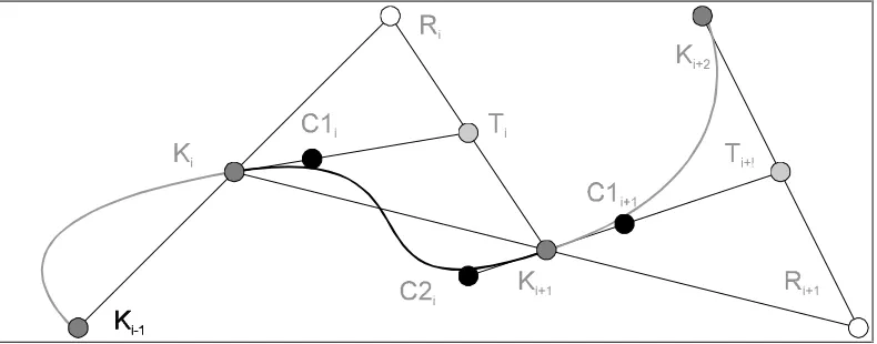
The following diagram shows the construction of inner control points for a Bézier segment in 2-dimensional vector space :

1

For example, if there is a key-frame (K1) at time 30, another (K2) at time 40, and a third (K3) at time

45, the camera will seem to suddenly speed up as is passes over K2. Although it is travelling at the

same velocity with respect to the Bézier parameter on either side of K2, the relationship of this

parameter to “global time” is different for each segment - both are parametrised from 0 to 1, but the first segment covers ten time units while the second only covers five.

2

G0 continuity means that the endpoints of two curves are coincident. G1 continuity means that, in addition to the endpoints being coincident, the geometric slopes of each curves at the join point are equal. C1 continuity means that the tangents (the first derivatives of the curves with respect to a global parameter) to each curve at the join point are equal (i.e. : both in direction and magnitude) - in general,

C1 continuity implies G1 continuity, except in the special case where the tangents are of zero length. Cn continuity implies that all derivatives of the curves through dn/dtn are equal on both sides of the join point. See [Fole90], pp 478-490 for further discussion on this topic.

3

Interpolate[x,y](u) should return an object which is conceptually along the “line” between x and y by the ratio u, such that Interpolate[x,y](0) = x and Interpolate[x,y](1) = y. For any linear space (in particular, in vector space), Interpolate[x,y](u) can be defined as x + u(y - x). For the space of rotation quaternions, it is (y x-1)u x, which performs great-circle interpolation of the quaternion along the surface

Figure 1: Bézier’s construction of inner control points

Bearing in mind that the inner control points of a Bézier curve define the tangents at the endpoints, it is clear that this construction generates endpoint tangents which are the mean of the vectors from the previous key position and to the next key position.4 If this construction is applied piecewise to all of the segments in the curve, the result is a smooth interpolant of the key points which is C1 continuous - i.e. it does not contain any sudden changes in direction or “velocity” with respect to the Bézier parameter.

Selecting an Initial and Final velocity

There are two points at which it is not possible to carry out the above construction, at the first keyframe K0, where there is no “incoming” direction, and the last keyframe Kn,

where there is no “outgoing” direction. A number of possible solutions exist to this difficulty :

• Set the initial/final velocity to zero (C10 = K0, C2n-1 = Kn) • Allow the user to arbitrarily select an initial/final velocity • Calculate the velocity depending on the rest of the segment

The first two options are self-explanatory, the third requires a little more explanation. It is possible to select a “reasonable” initial/final velocity for the first and last segments of the curve based on the tangent at the other end of the segment. One method of doing this is to construct a Bézier quadratic curve (rather than a cubic curve) using the two endpoints and the known endpoint tangent (a quadratic curve has one less degree of freedom than a cubic, so only three pieces of information are required to construct it, as opposed to the four which are required to construct a cubic) and then “lifting” this to cubic form. The details of this construction are omitted for brevity, but the resulting equations are :

C Interpolate K Interpolate K C C _n Interpolate K Interpolate K_{n n} C _n

1 2

2 1

0 0 1 0 32 23

1 1 1 32 23

= =

− − −

[ , [ , ]( )]( )

[ , [ , ]( )]( )

4

The vector KiTi is the actual tangent vector - the inner control points are placed 1/3 of the way along

this vector to generate a Bézier cubic curve with the required tangents. The fraction 1/3 arises from the

Evaluation of the Bézier Cubic Curve

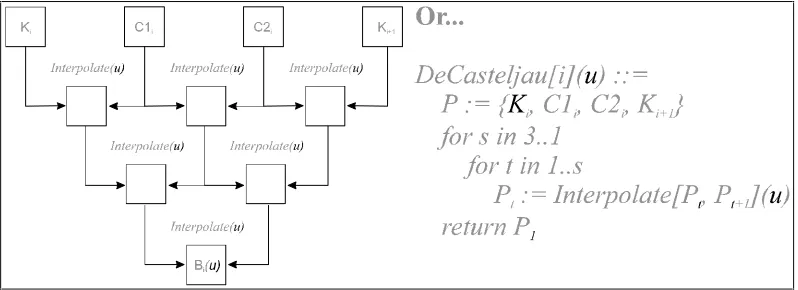
Once the four control points are known for each Bézier segment (the outer control points are the endpoints of the segment, the inner ones, defining the tangents at the endpoints, can be calculated as above), the Interpolate function can be used to evaluate the curve at any point along its length, using the technique of De Casteljau evaluation -to find the point Bi(u) on segment i, where u runs from 0 to 1 along the length of the

segment :

Figure 2 : De Casteljau evaluation

Note that this evaluation method only uses the Interpolate function and does not make any assumptions about other operators being defined on the space in question - this is important when dealing with quaternion space because other Bézier evaluation methods may not work in this space, or may not give the required result (because the sum of two quaternions does not represent the combination of the two rotations they represent). Note also that for a cubic Bézier curve (four control points), six calls to the Interpolate function are required.

Evaluating in “Global Time” space

If the interval between key-frames is constant at v time units, and the first key-frame K0

is at global time g = 0, then the position at any time g can be calculated as :

( )

_{ }

P g B g v

g v gv

= ( − )

Non-Constant Keyframe Intervals

The situation becomes significantly more complex if the time intervals between keyframes are not equal. Firstly, computing the segment number and Bézier parameter for a given point in global time can no longer be achieved by simply dividing by the inter-keyframe interval as above, but must be achieved by scanning through the list of keyframes - if KTi is the time for keyframe Ki with KT0 = 0 as before, then :

P(g) ::= i := 0

while g >= KTi

i := i + 1

Secondly, and more seriously, Bézier’s construction to achieve tangent continuity across keyframes relies upon the segments on either side of a keyframe having the same parametrisation with respect to global time. If the intervals between keyframes are not constant, the parametrisation becomes uneven, and the tangent continuity is lost.

To overcome this problem, a new method of constructing the inner control points is required; a method which takes into account possible variations in the intervals between keyframes. In order to generate such a method, it is necessary to return to Bézier’s original construction and investigate how it may be adapted.

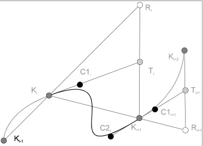
To generate the tangent vector at keyframe Ki, the mean of the “incoming” direction K

i-1Ki and the “outgoing” direction KiKi+1 is used. When the two segments are of different

lengths in global time space, it is no longer appropriate to use these vectors directly -rather, it is necessary to scale them so that they are appropriate to the parametrisation of the segment in question.

If the parametrisation ratios PRi are defined (for all keyframes except K0 and Kn) as

follows :

PR KT KT

KT KT

i i i

i i

= −

−

+ − 1

1

(i.e. : the ratio of the “speed” of the segment on the left to that of the segment on the right), the new construction equations for the Bézier control points, taking these ratios into account, are as follows :

R Interpolate K K PR T Interpolate R K

C Interpolate K T C Interpolate K C

i i i i

i i i

i i i

i i i PRi

= +

= = =

− +

+ + − +

[ , ]( )

[ , ]( )

[ , ]( )

[ , ]( )

1

1 12 1

3

1 1 1

1

1

2 1

1

Clearly, the amount of extra computation involved in this method is trivially small, especially when it is understood that this construction only need be performed once for a given list of keyframes. (The Bézier Quadratic construction given above for the initial and final velocities at the endpoints of the curve (K0 and Kn) does not need to be

changed to take variable parametrisation into account, because it operates entirely within the first and last segments.)

Figure 3 : Construction of inner control points with variable parametrisation

Higher-Order Continuity

The above system can be used to generate an interpolation curve which is C1 continuous at all points along its length - it contains no sudden changes in velocity at any point. This implies that the acceleration of a point, moving along the curve, is finite at all points (to remove ambiguity, the acceleration is defined as the second derivative of the Bézier curve with respect to global time : dP(g)/dg); however, the acceleration is not continuous, but has a discontinuity at each join point. This is a sufficient degree of continuity for most animation animations, because discontinuous accelerations are feasible in the real, physical world; however it may sometimes be desirable to construct curves with higher orders of continuity - specifically, with continuity of acceleration (C2 continuity).

Unfortunately, matching the accelerations of two Bézier cubic curves at their join point is extremely difficult, because Bézier cubics only have four control points, which specify the end points and the end velocities - there is no way to control the accelerations at the endpoints without affecting the velocities. If independent control of the end positions, the end velocities and the end accelerations is required, the smallest degree of curve which can be used is a quintic (5th order) curve, with six control points.

The six control points (C0 to C5) in a quintic curve determine the positions, velocities

Q C

Q C

Times Diff C C Times Diff C C

Times Diff Diff C C Diff C C

Times Diff Diff C C Diff C C

dQ dt dQ dt d Q dt d Q dt ( ) ( ) ( ) ( ( , ), ) ( ) ( ( , ), ) ( ) ( ( ( , ), ( , )), ) ( ) ( ( ( , ), ( , )), ) 0 1 0 5 1 5 0 20 1 20 0 5 1 0 4 5

2 1 1 0

3 4 4 5

2 2 2 2 = = = = = =

Notice the new functions Times and Diff which have been introduced. These functions are used instead of the more familiar algebraic operators to ensure that the equations can be used in spaces where linear arithmetic does not apply - specifically, in quaternion space. Times(X,m) returns an object which is “the result of applying X, m times” - in vector space, Times(X,m) := mX, and in quaternion space, Times(X,m) := Xm. Diff(A,B) returns an object which is the “difference” of A and B in vector space, Diff(A,B) := A -B, and in quaternion space, Diff(A,B) := AB-1. The proportions 5 and 20 appear because of the relationships between the control points of the quintic and the first and second differentials - derived by simple differentiation of the Bézier functions with respect to the parameter.

If another function, Sum(A,B), is introduced, such that Sum(A,Diff(B,A)) = B, the reverse calculation can be used to generate the six control points, given the two end positions (P0 and P1), velocities (V0 and V1) and accelerations (A0 and A1), as follows (In

vector space, Sum(A,B) := A+B and in quaternion space, Sum(A,B) := BA) :

C P

C Sum Times V C

C Sum C Sum Diff C C Times A

C P

C Sum Times V C

C Sum C Sum Diff C C Times A

0 0

1 0 15 0

2 1 1 0 0 120

5 1

4 1 15 5

3 4 4 5 1 120

= = = = = = ( ( , ), ) ( , ( ( , ), ( , ))) ( ( , ), ) ( , ( ( , ), ( , )))

The only remaining problem is : how are the Vn and An to be calculated? A suggested

method is as follows :

• Generate the “ordinary” cubic Bézier curves with compensation for variable parametrisation, as detailed above.

• Differentiate each segment of the resulting curve (twice) to get V0, V1, A0 and

A1 for that segment.

• At each join point, take the mean of the incoming A1 and the outgoing A0

(compensating as usual for variable parametrisation)

• Construct the quintic curve for the segment using this information.

5 for a quintic curve ) is equal to Times(Diff(C1,C0),n) and that A0 is

Times(Diff(Diff(C2,C1), Diff(C1,C0)),n(n-1)).

The final construction of the control points (C0,i to C5,i) a quintic Bézier curve between

two keyframes Ki and Ki+1 in an animation sequence, given the list of key positions Ki

and the list of parametrisation ratios PRi, as before, is as follows :

R Interpolate K K PR T Interpolate R K

x Interpolate K T y Interpolate K x

A Diff Diff y x Diff x K A Diff Diff x y Diff y K A Interpolate Times A PR A

A Interpolate A Times A

i i i i

i i i

i i i

i i i PR

i i i i i

i i i i i

i i i i

i i i i

i = + = = = = = = = − + + + − + − + [ , ]( ) [ , ]( ) [ , ]( ) [ , ]( ) ( ( , ), ( , )) ( ( , ), ( , )) [ ( , ), ]( ) [ , ( , ' , ' , ', ', , , , 1

1 12 1

3

1 1 1

0

1 1

0 1 1 0 12

1 0 1 1 + + + − + + + = = = = = =

1 1 12 0

1 15

2 1 1 0 0

3 4 4 5 1

4 1 1 1 1

5 1 1 1 ' , , , , , , , , , , , , , , , , )]( ) [ , ]( ) ( , ( ( , ), )) ( , ( ( , ), )) [ , ]( ) PR i i

i i i

i i i i i

i i i i i

i i i PR

i i

i

i

C K

C Interpolate K T

C Sum C Sum Diff C C A C Sum C Sum Diff C C A C Interpolate K C

C K

Notes : Ri and Ti are the same points as in the previous construction (the continuation of

the vector from the previous key position to the current one, and the calculated tangent vector, respectively). xi and yi are temporary variables, used in calculating the

accelerations (these are the same as the inner control points in the construction of the cubic). A'0,i and A'1,i are the calculated incoming and outgoing accelerations for the cubic

curve which would be constructed on this segment - the accelerations for the quintic (A0,i and A1,i) are calculated based on the mean of the incoming and outgoing cubic

accelerations. The six control points (C0,i to C5,i) are then computed using the identities

given above.

Once again, it is important to note that only the functions Times, Interpolate, Diff and Sum are used - provided these are defined appropriately, this technique can be used to give a smooth interpolant of key-positions in any space, giving C2 continuity with respect to a global time parameter. Definitions of these functions have been presented for vector and quaternion space; they should be easily extensible to cover other spaces as required.

Evaluation of the Bézier Quintic Curve

points in the initial list as opposed to four. The following Mathematica [Wolf91] definition will evaluate a Bézier curve at any point using the recursive De Casteljau algorithm - the control points are passed as the list a (Interpolate must be defined on the members of this list) and the Bézier parameter is passed as the scalar u :

Bezier[{x_}, u_] := x Bezier[a_, u_] := Bézier[

Table[Interpolate[a[[i]], a[[i+1]], u], {i, Length[a]-1}], u

]

Examples :

Interpolate[a_, b_, u_] := u b + (1 - u)a

Bezier[{{0,0},{1,1},{2,0},{4,2}}, 0]

=> {0, 0}

Bezier[{{1,0,3},[1,1,2},{3,4,0},{-1,1,-2},{2,0,0},{3,1,0}}, 0.75]

=> {1.51855, 0.867187, -0.495117}

The first example evaluates a point on a Bézier cubic curve in 2-d vector space, and the second evaluates a point on a Bézier quintic curve in 3-d vector space.

Advantages and Disadvantages of Bézier Quintic Curves

The Bézier quintic curve shares many of the advantages of the better-known Bézier cubic. In particular, the ease and efficiency with which the cubic curve can be evaluated, differentiated and integrated are largely maintained in the quintic, as the following table shows :

Operation Bézier Cubic Bézier Quintic

Evaluation at a point 6 Interpolate operations 15 Interpolate operations Differentiation with

respect to parameter

3 Diff operations and 3 Times operations

5 Diff operations and 5 Times operations Integration with respect

to parameter

4 Sum operations and 4 Times operations

6 Sum operations and 6 Times operations Storage requirements 4 control positions 6 control positions

Clearly, the quintic does not require vastly more computation time or storage resources than the cubic, and its greater flexibility in allowing both the first and second derivatives of the curve at the endpoints to be independently set is an important advantage when constructing piecewise curves with C2 continuity, as has been shown. On the other hand, the 150% increase in evaluation time might be regarded as too great a sacrifice to pay for the relatively small gain of C2 continuity in applications where it might not be required. In addition, the fact that it is a 5th order curve has implications for the overall shape - the possibility of unwanted “wiggles” being introduced is always present, and difficult to guard against.

as extensively investigated as other splines, in particular the B-spline and β-spline, and of course the traditional cubic Hérmite and Bézier cubic splines. Consequently, there may be hidden infelicities associated with the use of quintic curves which are not immediately apparent. In addition, the concept of using Bézier curves in spaces other than vector space has not been well-explored, so there may be pitfalls in that direction, too.

Conclusion

A generalisation of the Bézier algorithm for interpolation between keyframes is presented, allowing the following :

• Interpolations may be carried out in any space (not just vector space), provided a few simple manipulation functions are defined.

• It is possible to use keyframes which are not separated by constant intervals of global time.

• It is possible to generate curve segments with orders of continuity higher than C1, in particular, C2 continuity is reasonably simple to achieve. • Many advantages of the traditional cubic Bézier curve are retained, in

particular, compact representation, rapid evaluation, ease of differentiation and integration and “intuitive” representation.

This generalisation of the Bézier algorithm means that it is possible to use the well-known Bézier curves to construct smooth paths for an animation, with all the concomitant advantages. In particular, this extension allows the same algorithm to be used to interpolate between both the position and orientation components of a camera keyframe. The algorithm is not restricted to providing a smooth path for a virtual camera, but could be used to smoothly interpolate between a set of points in any space with respect to an arbitrary parameter.

Future Work

Further investigation into the properties of higher-order Bézier curves is required - in particular, into the properties of Bézier curves in quaternion space - do these curves have any specific “meaning” analogous to the physical system which corresponds to other splines? ([Fole90], pp 478-516)

It is possible to set up keyframes which result in “unreasonable” situations, where the camera will accelerate or decelerate at a very high rate, or where the curve develops unexpected kinks - heuristics should be developed to detect these situations and warn the user.

The paradigm is easily extended to re-parametrise a sequence of key positions to a continuous parameter; this would be particularly useful in unifying sequences of key-frames drawn from different sources - for example, if two components of a scene were produced by different simulation packages, with different “frame rates”, they could be unified using this technique for each of the variables in the components.

Bibliography

[Bézi70] Bézier, P.E.

Emploi des Machines à Commande Numérique

Translated as Numerical Control, Mathematics and Applications John Wiley and Sons, Ltd. London, 1972.

[Fole90] Foley, J.D., van Dam, A., Feiner, S.K., and Hughes, J.F.

Computer Graphics : Principles and Practice

Addison-Wesley Publishing Company. Reading, Mass., 1990.

[Gord74] Gordon, W.J. and Reisenfeld, R.F.

Bernstein-Bézier Methods for the Computer-Aided Design of Free-Form Curves and Surfaces

In “Journal of the ACM”, Vol. 21 No. 2 (April 1974), pp 293-310 Association for Computing Machinery. New York, 1974.

[Mac92] Mac An Airchinnigh, M.

Quaternions for Rotation

In “Proceedings of the 1st Irish Computer Graphics Workshop”, pp 14-32 Trinity College, Dublin. Dublin, 1993.

[Morr92] Morrison, J.

Quaternion Interpolation with Extra Spins In “Graphics Gems III”, ed. Kirk, D., pp 96-97 Academic Press, San Diego, 1992.

[Shoe85] Shoemake, K.

Animating Rotation with Quaternion Curves

In “Proceedings of ACM SIGGRAPH”, Vol. 19 No. 3 (1985). pp 245-252 Association for Computing Machinery. New York, 1985.

[Wolf91] Wolfram, S.