Reliability updating in linear opinion pooling for multiple decision makers

(1)

Reliability Updating in Linear

Opinion Pooling for Multiple

Decision Makers.

A thesis submitted to the University of Dublin, Trinity College

in partial fulfillment of the requirements for the degree of

Doctor of Philosophy

Department of Statistics, Trinity College Dublin

March 2016

(2)

I dedicate this thesis to the memory of my friend Faith Wilder,

5th of September 1985 - 21st of February 2015,

(3)

Declaration

I declare that this thesis has not been submitted as an exercise for a degree at this

or any other university and it is entirely my own work.

I agree to deposit this thesis in the University’s open access institutional repository

or allow the Library to do so on my behalf, subject to Irish Copyright Legislation and

Trinity College Library conditions of use and acknowledgement.

The copyright belongs jointly to the University of Dublin and Donnacha Bolger.

Donnacha Bolger

(4)

(5)

Abstract

Accurate information sources are vital prerequisites for good decision making. In this

thesis we consider a multiple participant setting, where all decision makers (DMs) have

a collection of neighbours with whom they share their beliefs about some common

relevant uncertain quantity. When determining which course of action to follow a DM

takes into account all the information received from her neighbours. Over time, in

light of the returns observed from choices made, DMs update their own beliefs over

the uncertain event, and also adjust the degree of consideration that they afford to

the opinions of each neighbour based on the level of reliability that the information

they provide is ascertained to have. Much of this thesis is concerned with constructing

a method that incorporates both of these learning facets in a dynamic fashion. This

technique, termed the Plug-in approach, is motivated and derived, and attempts are

made to justify its use by consideration of some attractive properties it obeys, in

addition to studies conducted using both simulated and real data which compared its

performance to some rational alternatives. Generalisations of this method are also

provided to a setting where DMs specify their opinions nonparametrically rather than

using probability distributions, as well as in a group setting where utilities as well as

opinions must be amalgamated. Two subjective approaches are also briefly discussed,

(6)

(7)

Acknowledgements

First and foremost I wish to extend my heartfelt thanks to my supervisor, Dr. Brett

Houlding. Throughout my Ph.D. tenure he has been constantly encouraging, and

extremely helpful at indicating which ideas deserved further consideration and which

should be forgotten about. Brett guided me through my first foray into research, always

quick to offer an insightful remark and never too busy for one of my frequent trips across

the corridor to his office. He generously funded me to travel to conferences, allowing me

to learn, to meet other statisticians, and visit exciting locations (and Kildare). Brett

demonstrated that “a Liverpool fan whose company I actually enjoy” is not necessarily

a guaranteed oxymoron. I could not have asked for a better supervisor than him.

I next wish to thank the staff of the Statistics Department, who have constantly

offered advice when I sought it and been incredibly supportive of my research over

the last three years. I’ve greatly enjoyed having a cup of tea with them every day.

Special gratitude goes to Simon Wilson, who both supervised my undergraduate final

year project (and hence kindled my passion for statistical research) and pointed me

towards Brett when I mentioned my contemplation of postgraduate study. Without

his encouragement it is doubtful if I would have embarked down the Ph.D. road.

I feel tremendously fortunate regarding the company I have been able to keep

during my time in Trinity, in terms of the postdocs and fellow Ph.D. students I’ve

worked alongside. I consider Angela, Gernot, Cristina, Joy, Sean, Arthur and Arnab

all to be great friends. It was a great pleasure to share an office with Shane O’Meachair,

Shuaiwei Zhou and Thinh Doan - all of whom are true Dubliners in different ways, and

who make for great company and constant fun. Finally Louis Aslett and Jason Wyse

were two wonderful mentor figures, doling out insights and counsel about the world of

research and academia both inside and outside of the Lincoln Inn on Friday evenings.

(8)

-they’re my homeboys at home, who have supported me constantly over the last three

years. After a tough day at work it was always nice to have an evening of hanging

out with them to look forward to. I am not a superstitious person, but a lot of stars

aligned extremely conveniently for me both in the lead-up to and during my time as a

Ph.D. student, and the unscientific part of me would like to think that my late mother,

Bernie, had a non-negligible impact upon this. A lot of the effort that I put into my

work was in the hope of doing her memory proud, and I’d like to think that in some

small way I achieved that.

Finally, it is utterly inconceivable that this thesis would have come into being

without the ever-present love and encouragement of Livi Flynn. Several times over

the past few years I felt that the Ph.D. challenge was too great for me to handle - a

bottle of Brooklyn Lager and slice of pepperoni pizza with her invariably righted my

wrongs. She has more goodness and patience than anyone I have ever met, and is

unquestionably my (statistically significantly) better half.

(9)

List of Tables

2.1 Cross-tabulation of utilities for D and Θ. . . 18

2.2 Cross-tabulation of utilities for D={d1, d2, d3} and Θ ={θ1, θ2}. . . . 19

2.3 Cross-tabulation of utilities for D={d1, d2}and Θ = {θ1, θ2}. . . 22

3.1 Prior Information and DM Weights . . . 47

3.2 DM information for our financial example. . . 59

3.3 Optimal decisions for DMs at the first and second epoch . . . 59

3.4 Updated opinions, and weights, of DMs and Pooling Methods. . . 61

3.5 Success Proportions for Linear Pooling Methods . . . 62

4.1 Simulation Study Initialisation Information . . . 79

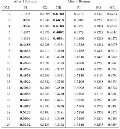
4.2 Group Success Proportions after three and four returns . . . 83

4.3 Individual Success Proportions after three and four returns . . . 84

4.4 Cross-tabulation of DMs and return streams . . . 87

4.5 TU Delft Expert Judgment Data Base details. . . 95

4.6 Differences between the Plug-in and classical methods. . . 96

4.7 Sample expert opinions . . . 96

4.8 Sample DM weights over time . . . 102

4.9 Individual problem success proportion. Optimal methods are in bold. . 104

4.10 Success proportions for the group problem. Optimal methods are in bold.105 4.11 Aggregated Individual Results . . . 106

4.12 Aggregated Group Results . . . 106

5.1 Sample DM utility information . . . 113

5.2 Original expected utilities of the DMs and the group. . . 119

(14)

5.4 Augmented Expected Utilities of P2 . . . 120

5.5 Original expected utilities of the DMs and the group. . . 121

5.6 The expected utilities of the DMs and the group. . . 123

6.1 Corresponding Values of ∆0 and ν . . . 131

6.2 Width vs. Accuracy merits . . . 135

6.3 Information at the first epoch . . . 138

6.4 First Weight Update . . . 139

6.5 First Opinion Update . . . 140

6.6 Information at the second epoch . . . 140

6.7 Second Weight/Opinion Update . . . 141

6.8 Success Proportions in Cases 1a-4a . . . 146

6.9 Success Proportions in Cases 1b-4b . . . 148

7.1 DM Information . . . 158

7.2 Weights from PI/DV methods . . . 158

7.3 Weights from PI/DV methods with fortunes doubled . . . 159

7.4 Change of Weights with ARA . . . 159

7.5 DM information for example. . . 160

7.6 Util Difference Between Predictions and Reality . . . 161

7.7 DM information for DV/PI comparison. . . 162

7.8 Weights from PI/DV methods . . . 163

7.9 Util Difference between PI/DV predictions . . . 164

7.10 DM information for DV/PI/KL comparison. . . 166

B.1 Original Expected Utilities of P1,P2 and the Group (P∗). . . 188

C.1 Success proportions: Normal overestimation in the group problem. . . . 191

C.2 Success proportions: Normal understimation in the group problem. . . 192

C.3 Success proportions: Normal mean-centred in the group problem. . . . 192

C.4 Success proportions: Poisson overestimation in the group problem. . . . 193

C.5 Success proportions: Poisson underestimation in the group problem. . . 193

C.6 Success proportions: Poisson mean-centred in the group problem. . . . 194

(15)

C.8 Success proportions: Binomial underestimation in the group problem. . 195

C.9 Success proportions: Binomial mean-centred in the group problem. . . 195

C.10 Success proportions: Normal overestimation in the individual problem. 196

C.11 Success proportions: Normal underestimation in the individual problem. 196

C.12 Success proportions: Normal mean-centred in the individual problem. . 197

C.13 Success proportions: Poisson overestimation in the individual problem. 197

C.14 Success proportions: Poisson underestimation in the individual problem. 198

C.15 Success proportions: Poisson mean-centred in the individual problem. . 198

C.16 Success proportions: Binomial overestimation in the individual problem. 199

C.17 Success proportions: Binomial undestimation in the individual problem. 199

(16)

(17)

List of Figures

2.1 Contrasting Utility Functions . . . 16

3.1 Prior Predictive Distributions/Plug-in Weights . . . 47

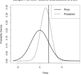
3.2 Normal Prior and Posterior Distributions . . . 50

3.3 Individual and combined distributions . . . 55

3.4 Illustration of Weights Convergence . . . 56

3.5 Prior Predictive Distributions . . . 60

3.6 Posterior Distributions . . . 61

3.7 Individual/PI Posteriors . . . 62

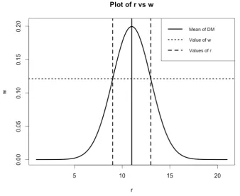
3.8 Plot of r vs. w . . . 64

3.9 Unnormalised plot of _P(Wi =wi|θ) . . . 65

3.10 Normalised plot of _P(Wi =wi|θ) . . . 66

4.1 The distributionsf1(θ)∼N(3,0.2) andf2(θ)∼N(−0.5,2), and θ = 1.8. 76 4.2 Optimal Methods in Normal overestimation . . . 80

4.3 Optimal methods for Binomial and Poisson overestimation. . . 80

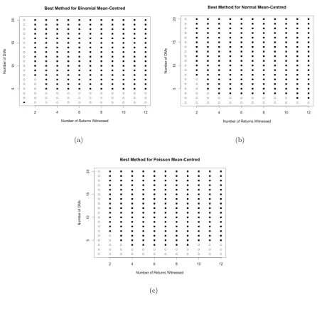
4.4 Optimal methods for Binomial, Normal and Poisson underestimation. . 81

4.5 Optimal methods for Binomial, Normal and Poisson mean-centred beliefs. 82 4.6 Simulated Proportions . . . 88

4.7 Simulation Proportions . . . 89

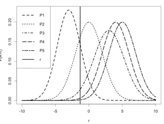
4.8 Prior Probabilities of PI Superiority . . . 91

4.9 Success probabilities for the PI, EQ and MR approaches for P2. . . 92

4.10 Fitted Cumulative Distribution Functions . . . 98

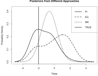
4.11 Posterior Distributions in Group Problem . . . 101

(18)

6.1 Prior and Posterior NPPIs . . . 131

6.2 Real line/Unit interval Prior and Posterior NPPIs . . . 138

6.3 Weights over time . . . 141

6.4 NPPIs over time . . . 142

7.1 PI/DV Posteriors . . . 163

7.2 Various Posteriors for DMs . . . 167

7.3 Weights allocated by DMs . . . 168

8.1 Social Network Illustration . . . 171

8.2 Two-period decision tree . . . 171

E.1 Poisson-Gamma Individual Convergence . . . 215

E.2 Poisson-Gamma Group Convergence . . . 216

E.3 Normal-Normal Individual Convergence . . . 218

(19)

Chapter 1 Introduction

When individuals make decisions they generally do so in the face of uncertainty.

Deci-sion makers (DMs, who are assumed feminine throughout this thesis) invariably have

some unsureness about the underlying process governing their decision environment,

e.g., they may not know the probability of a medical operation being successful, or

the number of cars that will pass along a motorway during rush hour. Generally the

language of probability is that used to express this uncertainty. It seems intuitive that

there is a connection between the accuracy of the relevant information that a DM

pos-sesses and the satisfaction that she will derive from the outcome resulting from the

decision that she makes. In this thesis we conjecture that it is beneficial for a DM to

absorb information from as many distinct sources as possible, and to assimilate these

into her decision process, incorporating additional knowledge into her task. Having

made a decision, a return is witnessed. We are concerned with two types of learning

that can subsequently occur. Firstly, a DM can update her own opinion about the

inherent decision uncertainty in light of this new evidence that has become available

to her. Secondly, she can reassess the respective perceived reliability of her various

information sources, who (in the context that we are concerned with) are a collection

of fellow non-competing DMs. Much of the work which follows aims at developing a

rational methodology that facilitates these two forms of learning and supplies a DM

with as accurate an opinion as possible to use in her decision task, as well as providing

justifications for the use of this approach in practice. We primarily assume individuals

specify their uncertainty via probability distributions, but we also provide an analogous

(20)

Above we have provided a broad outline of the original research that is contained

within this thesis. Below we supply detailed comments on the contextual setting that

this work is placed within, clearly outline the primary aims of the study conducted,

and highlight the research methodology that was adhered to throughout.

1.1 Contextual Setting

Every day important decisions with long-term repercussions are made. The United

Nations must reach resolutions on what actions to take concerning global conflicts,

governments of countries must determine how capital should be budgeted across their

departments, medical organisations must choose which drug trials should be funded

and which should not. In scenarios such as those illustrated above it seems unwise for

this decision to be made by a single individual, or at least to be made based solely

on the judgment held by one. A collection of people will generally possess a broader

knowledge span that a single person, and hence more pertinent information can be

incorporated into a decision making task by considering the opinions of a multiple

individuals. Additionally, on a practical basis, a crucial decision being made by one

person alone would lead to a great deal of accountability being placed on the shoulders

of that individual, something that can be lessened by a more collective process. Once

we concur that decision making via the amalgamation of several points of view holds

certain advantages over the alternative, the obvious question concerns the manner in

which such a decision should be made. In practical application there are numerous

methodologies that are likely to be employed.

Majority rule is an extremely straightforward approach, in which individuals vote

for their most favoured choice from a set of possible actions, with the action receiving

the greatest number of votes deemed to be best (in some sense) by the collective. This

is termed an ordinal decision scheme, with all emphasis explicitly placed on the

rank-ing order of decisions, rather than the degrees of preference inherent within individual

rankings and the ranking of the group as a whole. We shall return later in thesis

(no-tably in Section 5.4) to discuss the issues and potential pitfalls entailed within schemes

of this nature, but only comment now that they may not provide a complete picture

(21)

considered.

Different individuals will commonly hold diverse opinions based upon their

con-trasting degrees of knowledge over the uncertainty inherent within the forthcoming

decision to be made. Such contrasts may arise due to their potentially disparate

back-grounds; for instance their educational or socio-economic circumstances, how long they

have been involved with a particular organisation, if they have participated in a process

of this nature before, or if they have a vested interest in seeing a particular decision

chosen. Methods exist in which the individuals comprising a group will attempt to

bridge their intrinsic knowledge gaps by sharing their respective opinions and their

personal underlying rationales that led to their formations. Once they have listened

to the thoughts of those around them, individuals may potentially alter their own

opinions, perhaps conceding that they previously were ill informed about the topic at

hand and deferring to the wisdom of colleagues perceived to be wiser. Having done

this, the optimal decision is chosen by the group via discussion, which continues until

a collective consensus is happened upon. We shall further discuss methodologies of

this nature (known as behavioural methods) in more depth in our literature review of

Section 2, but for now only note that they too have complications ingrained within

them, perhaps most significantly being their susceptibility to biases and their potential

lack of rigour.

An obvious technique to be implemented is arguably the most democratic appearing

methodology, in which the opinions of all individuals are given an equal consideration.

On the surface there are certainly advantages apparent in approaches of this nature.

All participants are being treated equally, with no favouritism evident. The concept of

the wisdom of crowds is well known, with an averaging of opinions over an uncertain

quantity commonly leading to a more accurate estimate than if this was provided by

a single individual. Yet, as we shall discuss in our literature review of Section 2, and

numerous times in our findings of Section 4, there are clear foibles entailed in this

approach. If some individuals possess beliefs that are extremely inaccurate then these

have the potential to outweigh the beliefs of their more accurate peers, hence skewing

the collective opinion away from the truth. The greatest strength of this approach is

its simplicity of implementation, yet there are downsides that may occur as a result of

(22)

The clearest shortcoming of this equal weighting scheme is that the knowledge of

inaccurate individuals are given as much consideration as that of accurate individuals.

The easiest way to circumnavigate this would be to listen solely to the individual who

is deemed to possess the most reliable point of view, hence ensuring that unsound

opinions are discarded. Yet, even discounting our cautioning above about making

decisions based on a sole opinion, this leads to another major complication: how can it

be assessed who the most accurate individual is? All members of the collective believe

the opinion that they hold is accurate; if not they would not hold it, or would change

it to one that they felt was a more accurate reflection of the true state of nature.

It is extremely unlikely that any individual will willingly have their opinion discarded

entirely from the decision making task, especially considering that they may personally

believe it to be the most accurate of those proffered.

1.2 Research Aims

Given the above discussion concerning the contextual setting for our research, this

thesis can be seen as having three primary aims. First and foremost we aspire to

create an original decision making methodology, which takes steps towards solving the

complications that are inherent in the schemes discussed above. We mentioned the

shortcomings of decisions being made by a single individual, and hence our approach

shall be based upon the composition of a collection of (potentially diverse) opinions and

judgments from various sources. We commented on the issues inherent with behavioural

techniques, and therefore the scheme that we develop shall be strictly mathematical in

its formulation. An equal weighting scheme seems intuitive, but suffers from the fact

that accurate opinions may be outweighed by inaccurate opinions. However, at the

other end of the spectrum, it seems unwise to listen to a single individual deemed to

be most accurate, due to the complications in choosing such an individual, as well as

the aforementioned problem of basing a decision on a sole opinion. Hence our objective

is to create a method that accounts for the opinions of all individuals in an unequal

fashion. We aim to weight the opinions of individuals, and to set these weights as

proportional to the perceived level of knowledge of participants. Of course, as we shall

(23)

expand over the course of this thesis on reasons why our developed technique is indeed

truly original, and the advantages it can be seen to hold over existing alternatives.

Once we have developed a methodology of the nature discussed above our second

aim is to provide justification for its use in practical contexts. We want to be able to

pragmatically advocate for its application in realistic decision scenarios. It is our desire

for our approach to be mathematically logical, in the sense that it obeys properties

that a rational decision maker would deem important for an internally coherent decision

process to adhere to. Hence we intend to investigate the relationship between some

at-tractive statistical and mathematical attributes (for instance the Bayesian paradigm)

and our proposed methodology, and to confirm that this methodology does indeed

meet these criteria. In addition to justification by mathematical argument we also

want to provide data-driven validation, in order to highlight the practical merits of

our approach. We mentioned above that equal weighting, listening solely to the

indi-vidual deemed to be most reliable in a collective, and not taking any other opinions

into account at all are three frequently applied practices. We plan to compare the

performance of our methodology to each of these alternatives (using a suitably derived

comparative metric) to demonstrate the superiority of our technique. In Chapter 4

we see how this is achieved using a mix of simulated data and real world data. By

illustrating the merits of our approach against commonly used alternatives we hope to

underline the benefit of applying it in practical applications in order to increase the

quality of the decision process.

Our final primary aim is to provide some generalisations to our method, in order

to increase its flexibility and consequentially broaden the range of scenarios that it is

appropriate for usage in. Individuals may express their uncertainty concerned some

unknown commodity of interest in a variety of formulations, from a simple point

esti-mate to a fully parameterised probability distribution. Much of the work in this thesis

pertains to this latter case (with justification for this choice contained therein) but we

investigate in Chapter 6 if the general outline of our principal methodology can be

ex-tended to a significantly simplified setting, potentially increasing applicability (albeit

at the potential determent of the resulting decision quality). Arguably a strength of

the method that we derive is its rigid objectivity. However in Chapter 7 we develop

(24)

technique but that allow for different degrees of subjectivity to be entailed in their

mechanisms. These modifications, different flavours of our central methodology, allow

for our decision making scheme to be applied in a variety of contrasting settings rather

than a single specific one.

1.3 Research Methodology

We now progress to detail the research methodology that was followed during the

course of our research. Statistical decision theory has a rich history, formally dating

back at least as far as the 1730s. In order to be able to write knowledgably about

this topic, and the various nuanced subsets thereof, a reading of the seminal texts

was required. These are discussed in detail in the literature review of Section 2. We

began by consideration of the most basic decision making fundamentals (for instance

the notions of probability and utility), before expanding upon these in an incremental

fashion to explore increasingly deeper matters (such as decision making under imprecise

probabilities and the complications inherent within any group decision making scheme).

As indicated above, our foremost aim was in the development of a scheme suitable for

use in a decision context consisting of multiple individuals with differing degrees of

information about the uncertainty at hand. This concept of combining opinions or

judgments itself has an abundant amount of publications attributed to it. In Section

2.7 we thoroughly examine the most notable of these, highlighting ways in which they

contrast in their execution from what we desire, as well as detailing the contrasts

between them, and the various perceived advantages and disadvantages that they can

be said to hold over each other. The comprehensive literature review of Section 2 can

thus be seen as having a dual function: it provides the interested reader with enough

technical details and knowledge that they should be able to comfortably follow the

original research which it precedes, as well as providing adequate motivation for the

development of our novel decision making methodology.

It is in Section 3 that we derive this decision making methodology, explaining

comprehensively how weights (which represent the perceived accuracy of the decision

makers they are attached to) are calculated and updated over time, as well as how users

(25)

coher-ent fashion. Having produced our approach our desire was then to provide some formal

justification for it. We mentioned above that our approach is strictly mathematical,

rather than behavioural, and hence an obvious action was to assess its performance in

relation to some mathematical principles, and to see if it adhered to these. Crucially,

Section 2.6 contains discussion on how it is formally impossible to create a scheme that

can adhere to the entirety of a set of attractive criteria. Therefore we simply try to offer

a selection of desirable properties that our technique follows, without every making any

claims that these are indeed truly exhaustive. Section 3.2 delves into how our approach

fits into the Bayesian perspective, an important coherency property for those who wish

to adhere to this paradigm while updating weights/opinions over time. Section 3.5

presents four simple and attractive attributes that our method obeys. These pleasing

mathematical characteristics provide some initial basic justification for our technique.

As discussed in our aims earlier in this chapter it was our goal to provide a strong

justification for the method that we derive. The attractive coherency properties

cer-tainly are a step in this direction, but arguably not a full enough one. In order to

increase the rigorousness of our validation we strove to use data, and to compare our

technique to the aforementioned alternative approaches. An initial question concerned

the metric of comparison to be used. We consulted the seminal paper by Gneiting and

Raftery (2007) in order to be aware of the broad spectrum of possible metrics that could

be considered, eventually choosing one that we felt most appropriate for our setting.

Due to the novelty of our approach there were no pre-existing data sets constructed

in the commensurable fashion desired. Hence we simulated data to examine a broad

range of cases, varying the number of decision makers, the number of decision returns,

the confidence and accuracy of predictions, and the statistical distributions used to

represent these opinions. We compared our approach to the considered alternatives

under the chosen metric. The TU Delft Expert Judgment Data Base is a collection of

data sets that have arisen in realistic contexts, and have been used to provide

justifica-tion for one of the most commonly applied opinion pooling methodologies, the classical

method of Cooke (1991). Although the manner in which this data was collected does

not fully align with the required specifications of our context of interest we attempted

to suitably modify it in order to make it applicable for our approach. Having done this

(26)

data rather than simulated data, in order to strengthen the merits of our technique.

We briefly comment that methods of justification of the ilk discussed here are

repeated later in the thesis to deal with the various generalisations of our approach

that we develop: we consider a set of attractive properties that our group extension

obeys in Chapter 5, look at some axioms that our nonparametric approach in Chapter 6

adheres too in addition to consideration of a brief simulation study, before considering

some attractive coherency properties that our primary alternative subjective approach

in Chapter 7 obeys.

1.4 Outline of Thesis Chapters

We conclude our introduction with a brief summary of the the material contained in

the chapters of this thesis. In addition to this content there are several appendices,

highlighted in the main body of writing, that provide samples of code used, calculations

omitted, results summarised in the text, and tangential discussion points.

• Chapter 2 - Literature Review: The fundamental aspects of statistical decision

theory that will be used throughout this thesis are formally introduced. The

concept of precise probability is discussed, before the subtler notion of utility

theory is treated, as well as the relationship that exists between these two ideas,

and some additional comments on risk aversion. Maximisation of expected

util-ity is reviewed, with reference to its axiomisation and a brief numerical example.

Imprecise probability is then explored and a short numerical example given, as

well as discussion on how decisions can be made in the face of this additional

uncertainty, and a brief note on how expectation can be considered as a

primi-tive construct in lieu of probability. Group decision theory is then considered, as

well as the issues from Arrow’s Impossibility Theorem (Arrow, 1950) and notable

attempts to circumnavigate these. Finally, a detailed discussion takes place on

how a collection of opinions can be combined into a single opinion. The different

philosophies underlying methods of doing this are introduced, and the strengths

and weaknesses of various potential approaches supplied. Considerable attention

is paid to the classical method of Cooke (1991), and the TU Delft Expert

(27)

which we attempt to generalise in the following chapters.

• Chapter 3 - The Plug-in Approach: This chapter denotes the commencement

of the original research contained within this thesis. The notation used in the

remainder of the chapters is formally defined, and some further heuristic

justifi-cation provided for the concept of linear opinion pooling. The idea of Bayesian

updating is introduced, and discussion takes place in relation to three commonly

implemented conjugate cases which are used for illustration throughout. A

frame-work is supplied for decision making in the environment of interest, termed the

Plug-in (PI) approach. Details are provided regarding how individuals are

ini-tially given equal weights, before these are updated in light of their perceived

accuracy after returns are witnessed. A short numerical example demonstrates

PI weights in a Beta-Binomial conjugate setting. A discussion then takes places

relating to the Markovian elements of the PI process and two attractive Bayesian

properties it adheres to, as well as its relation to scoring rules. Some coherency

properties that the method obeys are examined, a detailed numerical example is

provided, and some asymptotic properties of weights and distributions are

men-tioned. Sample calculations are included regarding the distribution that weights

follow in the Normal-Normal conjugate case. The chapter also contains some

comments pertaining to the relatively straightforward extension of this approach

to a more generalised setting. We briefly compare our method with Bayesian

Model Averaging (Hoeting et al., 1999) and discuss some limitations on the

ap-plication of the PI approach.

• Chapter 4 - Data-based Justifications: Leading on from the somewhat informal

justifications of the PI approach in the previous chapter, we aim to provide

a more rigorous basis for its use. This is attempted using two types of data,

simulated and real. Data is simulated for the three distributional cases

previ-ously introduced, and the PI approach is compared to a collection of rational

alternatives under a particular probability density metric. We also provide the

theoretical calculations underlying these simulations, and demonstrate how our

simulated proportions asymptotically approximate the true probabilities of the PI

(28)

assessed using the previously introduced TU Delft Expert Judgment Data Base.

Discussion is provided on the contrast between the nature of this data and that

naturally arising within the PI approach, before rationalisation is provided for

the methods used to bridge these contrasts. The performance of the PI approach

is compared for each data set in turn to the performance of alternatives, with the

meaning of these results interpreted.

• Chapter 5 - Group Decision Making: This short chapter discusses how the PI

ap-proach can be applied in a group decision making context. This entails combining

utility functions as well as probability distributions, with commentary provided

on how this may be done in a manner ensuring commensurability (Boutilier,

2003). The proposed group decision making process is considered in relation to

each of the five axioms of Arrow (1950). The chapter concludes with comments

on the links between our method and Utilitarianism (Harsanyi, 1955), and the

merits of cardinal, rather than ordinal, decision ranking schemes.

• Chapter 6 - Nonparametric Extension: Up to this point it has been explicitly

assumed that DMs can supply fully parameterised probability distributions to

quantify their uncertainty, with the PI approach being reliant upon this premise.

Here we discuss how this assumption may be weakened, and consider a far more

simplistic method of nonparametric belief specification. The concept of

Nonpara-metric Utility Inference (Houlding & Coolen, 2012) is introduced. Arguments are

provided regarding how the rules of this method may be augmented for an opinion

updating scenario, where the opinions of a DM over the expectation of the

uncer-tain quantity are represented simply by intervals, referred to as Nonparametric

Prevision Intervals (NPPI). In the context that we consider here, expectation

(i.e., prevision) naturally arises as the obvious choice of primitive construct. A

weighting methodology that explicitly learns over time in multiple ways is

sug-gested, and a detailed heuristic justification is given for its use, invoking the

scoring rule discussed in Gneiting & Raftery (2007). A numerical example

illus-trates how this method may be used in practice. A suitable metric is proposed,

before a brief simulation study demonstrates the potential merit of our approach.

(29)

fully objective, in the sense that the weights it produces are based solely on

the data that is witnessed. In this short chapter two alternative methods that

incorporate considerable subjectivity are motivated and derived. The Differing

Viewpoints approach explicitly models the utility function of the individual

as-signing weights, with, for instance, a highly risk prone DM asas-signing a particular

prediction a substantially different weight than the weight assigned by deeply risk

averse DM. Some formal statements are provided in relation to the risk aversion

metric introduced in Chapter 2, and an appropriate performance metric is

de-tailed. The Kullback-Leibler approach, in which a DM assigns higher weights to

those individuals whose beliefs closely mirror her own, is briefly discussed and its

strengths and weaknesses examined. The chapter concludes with a short example

comparing the performance of the three original methodologies provided in this

thesis.

• Chapter 8 - Summary and Further Research: This final chapter of this thesis gives

a brief summary of the research conducted and the conclusions reached therein.

Various potential extensions for further work are offered. An application to a

social network setting is suggested, with a notation and linear opinion pooling

form provided. A discussion takes place about sequential decision problems,

most notably concerning the relation to the polynomial utility class (Houlding

et al., 2015), and its possible implementation in the setting from this thesis. A

method of decision making with constant learning is suggested using not only

imprecise probabilities (as in Chapter 6) but also imprecise utilities (for instance

over novel returns), allowing for additional uncertainty for users regarding the

specification of relevant quantities. Another idea for complementary research is

the introduction of a non-flat hierarchy inherent within a group (e.g., a

govern-ment), where the weight assigned to individuals incorporates their rank. We also

mention learning over time in relation to a series of correlated random quantities,

that are either realisations of distinct random variables (withθ potentially being

multivariate) or realisations of a single dynamic variable, rather than the static

quantity considered in this thesis. Links with the concept of value of information

(30)

(31)

Chapter 2 Literature Review

The two pillars upon which statistical decision making is built are probability and

utility, both of which shall be given substantial treatment in what follows. Initially we

focus on precise probabilities, but we will later turn our attention to imprecise

prob-abilities which shall become relevant in Chapter 6. We discuss maximising expected

utility as a decision making criteria, as well as the objections raised, and alternatives

proposed, to this approach. Comments are made regarding decision making

methodolo-gies in an imprecise setting. We analyse group decision making, issues associated with

implementing this fairly (in terms of Arrow, 1950), and some alternative approaches

put forward, which will be discussed again in Chapter 5. Lastly we review methods of

opinion pooling, referencing the various schools of thought on manners by which this

can be done, as well as advantages, disadvantages and justifications for these.

2.1 Precise Probabilities

Probability is a method of quantifying uncertainty. In a non-trivial decision making

framework uncertainty will be faced by a DM, who is unsure of the exact consequences

that will result from her decisions. Probability describes the unsureness of a DM

about the environment she inhabits. In this thesis we consider only DMs with

imper-fect knowledge, i.e., those who are unsure about some aspect of the true mechanisms

controlling their areas of interest,e.g., how a stock price fluctuates, or how many

pas-sengers will book a particular flight. Kolmogorov (1950) provides a strict axiomatic

(32)

provide these, where Θ is the space of all possible events, θ is a particular event, and

P(θ) is the probability of θ occurring.

• Axiom A1: Ifθ ∈Θ then_P(θ)∈_Rand _P(θ)≥0.

• Axiom A2: There is a universal event Θ∗ ⊆Θ such that _P(Θ∗) = 1.

• Axiom A3: For a set of countable mutually exclusive events θ1, θ2, . . . ∈Θ

P(θ1 ∪θ2∪. . .) =

∞

X

i=1

P(θi)

Further rudimentary properties can be derived from these, e.g., monotonicity and

bounds of probability. A set of probabilities failing to meet A1-A3 risks falling prey to

a “Dutch book” (e.g., Maher, 1993), which occurs when a DM enters a wager she is

doomed to lose irrespective of what outcome occurs. The probability associated with

the occurrence of an eventθcan be considered the price at which a rational DM would

be willing to buy (or equivalently sell) a bet that pays one util (shortly to be defined)

if θ occurs, and zero utils if not. When we discuss imprecise probabilities we shall see

an intuitive extension of this betting analogy.

2.2 Utility

2.2.1 Expected Value Theory

Early probability studies were centred on gambling, i.e., in determining how likely a

player was to win a game and what was a fair stake for them to pay to play. Arguably

the foundations of probability theory arise from a series of letters between Blaise Pascal

and Pierre de Fermat concerning a question posed to them by Chevalier de Mere

regarding a particular game of chance. A fair stake was often considered the expected

value of the outcome of playing the game. This method had shortcomings, highlighted

by Bernoulli (1738) in the St. Petersburg Paradox. This describes a game in which

a player tosses a fair two-sided coin, and wins a pot (doubling with each success) for

every consecutive toss resulting in heads. She receives the pot the first time she tosses

(33)

E, we find

E = 1 2×2 +

1

2

×22+

1

2

3

×23+

1

2

4

×24+. . .= ∞

X

k=1

1 = ∞

This is clearly a ridiculous choice of fair price, indicating that the expected prize from

playing is an infinite sum. Hence we see that expected value theory is not always

a logical decision making criteria, as here a player will give any finite sum to play.

Bernoulli used this argument to motivate a new decision making criteria.

2.2.2 Utility Hypothesis

Bernoulli (1738) wrote that “. . . the determination of the value of an item must not be

based on the price, but rather on the utility it yields. There is no doubt that a gain of

one thousand ducats is more significant to the pauper than to a rich man, though both

gain the same amount”. He said that DMs should specify their own utility functions,u,

that describe their personal attitudes over outcomes, risks and gambles. Formally u is

a function, u:R→_R, from the set of possible decision returns R, to the real numbers

R. For every possible decision a numerical value (measured in units called utils) can be

calculated, with the optimal decision returning the highest value, in a process formally

defined in Section 2.3.1. There are many advantages to this method in comparison

with expected value theory, e.g., it allows for personalistic interpretation of the merits

of outcomes. It will generally yield different numerical values (and hence decisions) for

different DMs depending on their utility functions, opinions and (in financial settings)

monetary situations. It can be argued as a more useful criteria than expected value

theory as it incorporates much more information into the decision making process.

2.2.3 Measures of Risk-Aversion

A DM’s utility function,u(r), measures the satisfaction she derives from returnsr∈R,

and reflects her attitude over gambles, i.e., if she is averse, neutral or

risk-prone, and to what degree. Suppose a DM has a fortune off units, and must determine

whether to play a game, raising her fortune tof +m units, or decreasing it to f −m

units, with probabilities of 0.5 respectively. Not playing the game has expected utility

(34)

• risk averse ifu(f)>0.5u(f+m) + 0.5u(f−m),i.e., she opts not to gamble, and

indeed would be prepared to pay to avoid taking the gamble.

• risk prone if u(f) < 0.5u(f +m) + 0.5u(f −m), i.e., she opts to gamble, and

indeed would be prepared to pay to take this gamble.

• risk neutral ifu(f) = 0.5u(f+m) + 0.5u(f−m), i.e., both decisions are equally

favourable, and she would neither pay to take or avoid taking the gamble.

A utility function that is risk-averse over a range is concave over this. Convexity

im-plies risk-proneness and a straight line imim-plies risk-neutrality, e.g., Fig. 2.1. Formal

measures exist to determine which classification a function falls under (and to what

degree), perhaps most commonly the Arrow-Pratt absolute risk-aversion (ARA)

coef-ficient, from Arrow (1965) and Pratt (1964), given by

A(r) =−u

00₍_r₎

u0₍_r₎ (2.1)

Fig. 2.1: Contrasting utility functions over the range [1,10]. From left to right we have (a) the risk-averse (concave) function u(r) = ln(r), (b) the risk-neutral (straight)

function u(r) = 2r+ 1 and (c) the risk-prone (convex) function u(r) =r3.

As two examples, u(r) = log(r) leads to A(r) = 1_r, positive for all possible values

of r (as logarithms take only positive input), implying risk aversion. By contrast,

u(r) = r3 yields A(r) = −2

r, indicating risk proneness/aversion for positive/negative

values of r respectively. Functions of the form u(r) = 1−exp(−αr) give A(r) = α,

(35)

A(r) = _ar1₊_b (for a, b ∈ _R) exhibiting Hyperbolic Absolute Risk Aversion (Merton, 1971). Higher order generalisations of ARA such as absolute prudence and absolute

temperance are discussed in Kimball (1990).

2.2.4 Relationship between Utility and Probability

We briefly mention the relationship that exists between utility and probability. Each

DM has a subjective utility function u(r). While in practice elicitation of this is

difficult, theoretically it is doable due to the “twinned” relationship of (subjective)

probability and utility, discussed in French (1994), whereby it is impossible to define

one without the other. The following two formal definitions illustrate this.

• Definition: A DM’s subjective probability for the occurrence of an event is the amountpshe is willing to gamble such that she receives 1 util if the event occurs,

and 0 utils if not.

• Definition: The utility a DM assigns to an outcomer is the value pmaking her indifferent between

(a) r for certain and

(b) a gamble between the best possible outcomer∗, withu(r∗)=1, with probability

p, and the worst possible outcomer∗, with u(r∗)=0, with probability 1−p.

In this utility definition the values are rescaled to the unit interval. We discuss why

this is possible in Section 2.3.3. Circularity can be noted between the two definitions.

It seems justifiable for French (1994) to refer to utility as “probability’s younger twin”.

Note both concepts are derived from the preference relation ordering,, that we shall

shortly define.

2.3 Expected Utility

2.3.1 Decisions

We denote a set of potential decisions by d1, d2, . . . , dn ∈ D, where D is the set of

admissible decisions, and each di is a distinct action. The satisfaction derived from a

(36)

uncertain over which state will obtain. For example, the merits of a trip to a restaurant

are dependent upon whether the chef is a good cook or not. One of these states is true,

but a DM is uncertain which one it is prior to choosing to eat there. Suppose there are

m potential mutually exclusive and exhaustive states of nature, θ1, θ2, . . . , θm ∈Θ. A

DM states her utilities over all possible outcomes (Table 2.1), where u(di, θj) denotes

the utility resulting from making decision di and the occurrence of θj.

Table 2.1: Cross-tabulation of utilities for D and Θ.

θ1 θ2 . . . θm

d1 u(d1, θ1) u(d1, θ2) . . . u(d1, θm)

d2 u(d2, θ1) u(d2, θ2) . . . u(d2, θm)

..

. ... ... ... ...

dn u(dn, θ1) u(dn, θ2) . . . u(dn, θm)

The expected utility of a decisiondi is the sum over the products of the probability

of each possible return occurring and the utility value associated with this, i.e.,

E[u(di)] = m

X

j=1

u(di, θj)P(θj) (2.2)

This sum is replaced by an integral if returns and/or probability distributions over

returns are continuous. The optimal decision,d∗, maximises Equation (2.2), i.e.,

d∗ = arg max

i E[u(di)] (2.3)

Lindley (1991) comprehensively treats this approach. In the framework discussed

here, it is assumed that DMs can both probabilistically quantify uncertainty over

po-tential returns and specify exact utility values corresponding to these. Realistically

this may often not be the case. In the absence of these abilities elicitation methods

exist to help discover these unknowns,e.g., the techniques of O’Hagan (1998) are often

used for belief elicitation. Regarding utility, a method by which preferences can be

ascertained over time is adaptive utility, discussed in,e.g., Cyert and DeGroot (1975),

and Houlding & Coolen (2011), and modified to incorporate extreme vagueness in the

priors over parameters in Houlding & Coolen (2012). Chajewska et al. (2000) also

(37)

2.3.2 Example using Precise Probabilities

A DM must choose whether to play football (d1), rugby (d2) or snooker (d3). There are

two possible mutually exclusive states of nature: the weather will be sunny (θ1) or rainy

(θ2), with Table 2.2 containing her utilities. Suppose she assessesP(θ1) = 0.7 implying

P(θ2) = 0.3. Using Equation (2.2) she finds that E[u(d1)] = 0.73, E[u(d2)] = 0.48 and

E[u(d3)] = 0.7,i.e., her optimal decision isd1, to play football.

Table 2.2: Cross-tabulation of utilities for D={d1, d2, d3} and Θ ={θ1, θ2}.

θ1 θ2

d1 1 0.1

d2 0.6 0.2

d3 0.7 0.7

2.3.3 The axiomatisation of von Neumann and Morgenstern

The work of von Neumann & Morgenstern (1944) axiomatically justified utility theory.

They created four rational axioms. If a DM agreed with these, and was herself rational,

then she would make decisions by maximising expected utility. These axioms are:

• Completeness: For any d1, d2 ∈ D, a DM can always determine which, if either,

she prefers, i.e. either d1 d2, or d2 d1. The relation implies weak

pref-erence, with d1 d2 stating d1 is at least as preferable as d2. Indifference is

indicated byd1 ∼d2, with denoting strict preference.

• Transitivity: If d1 d2 and d2 d3 then d1 d3, for all d1, d2, d3 ∈ D. This

ensures “money-pump” situations cannot arise.

• Continuity: Ifd1 d2 d3then there isp∈[0,1] withd2 ∼pd1+g(1−p)d3for all

d1, d2, d3 ∈D, i.e., there exists a probabilityp making a DM indifferent between

a gamble between the best and worst outcome (with probabilities p and 1−p

respectively) and a guaranteed intermediate outcome. Note that the operator +g

(38)

• Independence: If d1 d2 and p ∈ [0,1] then, for any alternative d3, we must

have pd1+g (1−p)d3 pd2 +g (1−p)d3 for all d1, d2, d3 ∈D, i.e., preference is

invariant to the introduction of independent alternatives.

Von Neumann and Morgenstern showed for a DM agreeing with these that there is a

unique (up to positive linear transformation) utility function such that:

• u(d1)≥u(d2) if and only ifd1 d2 for all d1, d2 ∈D.

• For all d1, d2 ∈D, and anyp∈[0,1],u(pd1+g(1−p)d2) =pu(d1) + (1−p)u(d2).

Hence a formal justification was given for maximising expected utility, advocating it

as a method for DMs deemed rational in some sense. Expanding on the invariance of

utility functions to positive linear transformations, a DM need not be concerned if she

specifies her utility function as u1(d) or u2(d) = au1(d) +b for a, b ∈ R and a > 0,

i.e., the decision deemed optimal under u1 is optimal underu2, and the converse. This

property arises due to the linearity of the expectation operator over its arguments.

2.3.4 Objections and Alternatives

The above method is normative,i.e., providing a formal method by which rational DMs

should make decisions. Yet human beings are prone to irrationality and not always

behaving in a manner consistent with this. The Allais paradox illustrates the decision

making irregularity often exhibited by DMs (Allais, 1953). DMs were questioned on

what decisions they would make in two separate hypothetical situations. The first

question asked if DMs would rather have $1,000,000 with certainty (A1), or $1,000,000

with probability 89%, $5,000,000 with probability 10% and $0 with probability 1%

(A2). The second question asked if DMs would rather have $1,000,000 with

probabil-ity 11% and $0 with probabilprobabil-ity 89% (B1) or $5,000,000 with probabilprobabil-ity 10% and $0

with probability 90% (B2). The most common pair of decisions to choose was A1 and

B2. This is inconsistent with utility theory, under which choosing A1 implies

automat-ically choosing B1, and choosing A2 implies automatautomat-ically choosing B2. Irrespective

of the utility function given by a DM it is impossible, under the framework of von

Neumann and Morgenstern, to choose both A1 and B2. This is presented by Allais as

(39)

A2, and B1 and B2, is a common increase in the probability of receiving $0, violating

this axiom.

An attempt to resolve this problem was the development of descriptive decision

making methods, describing how DMs actually make choices and incorporating human

characteristics, perhaps most notably Prospect Theory (Kahneman & Tversky, 1979).

This attempted to mirror behaviour exhibited by DMs in realistic scenarios, such as

how they feel the pain of a loss more severely than the joy of an equivalent gain,

and how they underweight outcomes that are probable compared to those that are

guaranteed. Fuzzy logic (Zadeh, 1965) modifies classical set theory, allowing items to

belong to several distinct sets at once with varying degrees of membership. Statements

need not be strictly true or false, but may have truth values in the [0,1] interval. There

are advantages to this approach but, as we shall shortly see in decision making under

imprecise probability, computationally it has significant disadvantages.

2.4 Imprecise Probabilities

Supplying a precise probability is a strong statement, implying that a DM knows

enough about the unknown quantity to exactly quantify her uncertainty over it. DMs

may have relevant prior experience, or expert advice, to help them do this. What

should a DM do if shea priori has little relevant information about the topic at hand?

Precise probability statements play a vital part in determining optimal decisions,e.g.,

in Section 2.3.2 using _P(θ1) = 0.7 led to d1 being chosen, yet slight augmentation to

P(θ1) = 0.65 makesd3 optimal. DMs must be careful in supplying precise probabilities

as, if inaccurate, they may lead to negative (low utility) consequences. An alternative

is the concept of imprecise probabilities. Rather than a single probability value _P(θ), a DM gives a lower bound _P(θ), and upper bound ¯_P(θ), that she maintains _P(θ) lies within. Probability measures uncertainty, with imprecise probability allowing

addi-tional vagueness. Analogous to Kolmogorov (1950), there are imprecise probability

axioms (Weichselberger, 2000, 2001), B1-B3. It is assumed_P(θ) obeys A1-A3.

• Axiom B1: 0≤_P(θ)≤_P¯(θ)≤1 for all θ∈Θ.

(40)

• Axiom B3: inf_P{_P(θ)}=_P(θ) and sup_P{_P(θ)}= ¯_P(θ).

From these further properties can be garnered. Denoting by θc _{the complementary}

event of θ we have ¯_P(θc_{) = 1}₋

P(θ) and P(θc) = 1 −P¯(θ). Previously we gave a

betting price interpretation to precise probabilities. There is an attractive analogy for

imprecise probabilities, with the lower bound probability being the smallest price for

which a DM is willing to sell a bet (in which she must pay one util if θ occurs and zero

utils if not) and the upper bound probability being the largest price for which she is

willing to buy a bet (in which she receives one util if θ occurs and zero utils if not).

Imprecise probability theory is an expanding topic, with many techniques constructed

for tasks that formerly required precise probabilities, e.g., Walley (1991) and Coolen

et al. (2010).

2.4.1 Decision Making using Imprecise Probabilities

How can DMs determine optimal decisions when opinions about θ are given by

im-precise probabilities? Consider Table 2.3, with a DM assessing _P(θ1) = 0.4 and

¯

P(θ1) = 0.6. For P(θ1) = 0.55 she deems d1 optimal, P(θ1) = 0.45 means d2 is optimal

and _P(θ1) = 0.5 gives a tie. Her optimal decision depends upon which probability (in

her range) is considered when calculating expected utilities. Often a single decision

cannot be declared unanimously optimal under all imprecise configurations.

Table 2.3: Cross-tabulation of utilities for D={d1, d2} and Θ ={θ1, θ2}.

θ1 θ2

d1 1 0

d2 0 1

If a single decision cannot be declared optimal it is important to eliminate decisions

that are unequivocally not optimal, i.e., inadmissible (e.g., Coolen, 2006). If a DM

cannot pick one alternative as maximal then she may choose a decision by a chance

mechanism, akin to uniform preference over decisions. It is desirable to omit as many

inadmissible decisions as possible before making this choice. We discuss four common

decision making methods for imprecise probabilities, two which choose an optimal

(41)

in Schervish et al. (2003), these methods can be seen as coherent, i.e., avoiding Dutch

books. If a decision has maximal expected utility under all belief configurations it is

optimal. This will frequently not be the case, but if it is then this decision choice is

robust. In a precise setting, Maximin (Wald, 1950) chooses the decision returning the

largest minimum expected utility value, i.e., a pessimistic approach. Γ−Maximin is

an imprecise probability extension of this. Maximality (Condorcet, 1785) eliminates

inadmissible decisions, i.e., those giving lower values than an alternative for all

con-figurations. E-Admissibility (Levi, 1974) removes all decisions from D except those

which are optimal under at least one belief specification. The set of decisions left after

applying E-Admissibility is a subset of that remaining after Maximality.

For the problem in Section 2.3.2, suppose _P(θ1) = 0.3 and ¯P(θ1) = 0.7,

imply-ing _P(θ2) = 0.3 and ¯P(θ2) = 0.7. Maximising expected utility is inconclusive. The

Γ−Maximum values ofd1,d2 and d3 are 0.37, 0.32 and 0.7 respectively,i.e., under this

criteria d3 is optimal. Maximality shows both d1 and d3 dominate d2, so it is

elimi-nated, while under E-Admissibility d1 is optimal for 2₃ <P(θ1)≤0.7 andd3 is optimal

for 0.3≤_P(θ1)< 2₃. There is no configuration makingd2 optimal, so it is eliminated.

2.4.2 Choosing a Primitive Quantity

Probability is often used in statements of uncertainty. In deriving axioms and theorems

the concept of a probability is usually considered “the primitive”,i.e., the fundamental

quantity upon which all further statements are built. If we are interested in the

ex-pectation of a random variable X, and have probabilities for its potential realisations

x1, . . . , xn then we define this expectation as

E(X) =

n

X

i=1

xiP(X =xi) (2.4)

This is not the only possible route. As in de Finetti (1974) and Whittle (1992) we can

take expectation as the primitive and define other concepts in terms of this. Consider

an indicator variableIX(xi), taking a value of 1 ifX =xi, and 0 if not. The probability

of xi occurring is then the expectation of this indicator variable, i.e.,

P(X =xi) = E[IX(xi)] (2.5)

Equation (2.4) defines expectation in terms of probability while Equation (2.5) did the

(42)

(e.g., Walley, 1991). In Chapter 6 this is the framework we adhere to.

2.5 Sequential Problems

The methods above considered a DM making a single decision, yet DMs often need to

make decisions for several future epochs simultaneously,i.e., non-myopically. In a

my-opic setting DMs consider one step into the future, at which time they observe a result,

and consider one step into the future again. A non-myopic setting is one in which a DM

must decide in May how much money she will need in June, July and August. These

problems are solvable using decision trees and the “roll-back” technique (Alghalith,

2012, proposes a “roll-forward” method), discussed via maximising expected utility by

Lindley (1991). An issue with this approach is the “curse of dimensionality”,i.e., when

a large amount of epochs and/or potential decisions are involved trees rapidly become

very complicated and computation is slow. Intractability may occur depending on the

form of probability distributions and utility functions. A method easing these issues

is the polynomial utility class (Houlding et al., 2015), reliant upon the assumptions of

polynomial utility functions and Normal probability distributions, creating conjugacy

for utility functions analogous to that existing for probability distributions. We return

to sequential problems in Chapter 8.

2.6 Group Decision Making

The approaches above dealt with a single DM making a decision, yet group decision

making is an important task too. While there is motivation for a normative method to

assist groups in making rational choices we shall see, for a certain set of axioms, that

this is an unobtainable goal due to the Impossibility Theorem of Arrow (1950). Efforts

have been made to circumnavigate this and find an acceptable group decision making

method, with strengths and weaknesses of some such approaches discussed below.

2.6.1 Arrow’s Impossibility Theorem

Arrow (1950) considered preference ranking among a body of individuals, and if there

(43)

ranking (). He contemplated a Social Welfare Function (SWF) operating on a set

of individual rankings, which would obey certain basic properties (completeness and

transitivity) and lead to a group ranking obeying the same. He put forward five

desirable axioms for this SWF to obey. Universality stated that the SWF be defined

for every admissible set of individual orderings. Monotonicity declared that if a decision

d1 rose, or did not fall, in the ordering of each DM without any other change in those

orderings, and ifd1 was preferred tod2 before the change to individual orderings, then

d1 is still preferred to d2. Non-imposition and non-dictatorship respectively ruled that

the SWF be neither imposed nor dictatorial. Independence is the most controversial

axiom. In a two DM setting, let1,2 and01,

0

2 be two sets of individual orderings.

If for both individuals i, and for all d1, d2 ∈ D, d1 i d2 if and only if d1 0i d2,

then the choice made is the same whether the individual orderings are 1 and 2, or

0

1 and 02. Monotonicity and non-imposition can be combined to form the Pareto

principle axiom (Arrow, 1963). Arrow (1950) showed that for at least two DMs and

three distinct decisions, no SWF satisfying the five conditions can be created,i.e., any

SWF is irrational in some sense. Independence is the axiom researchers most commonly

try to sidestep, as it assumes no preference between any two outcomes is stronger than

that between any other two outcomes, i.e., it is ordinal rather than cardinal. Several

other interesting impossibility results exist, e.g., May’s Theorem (May, 1952), the

Liberal Paradox (Sen, 1970), the Gibbard-Satterthwaite Theorem (Gibbard, 1973 or

Satterthwaite, 1975), and the Duggan-Schwartz Theorem (Duggan & Schwartz, 1992).

2.6.2 Utilitarianism and the SWF

Utilitarianism is a normative theory, broadly stating that well-being should be

max-imised and suffering minmax-imised. A leader, P∗, must translate the rankings of n

in-dividuals to one collective ranking. From two axioms a cohesive group ranking may

be achieved, as in Harsanyi (1955). All DMs assign utilities to each potential option,

scaled to [0,1], giving utility functions u1, . . . , un that must be translated to a single

function, u∗. The axiom of anonymity states thatP∗ does not know who put forward

which ranking, i.e., no bias. The second axiom is the strong Pareto principle,

declar-ing that if each individual is indifferent between two outcomes then so is P∗, i.e., if

Reliability updating in linear opinion pooling for multiple decision makers