Output Strictly Local Functions
Jane Chandlee University of Delaware
R´emi Eyraud QARMA Team
LIF Marseille remi.eyraud@ lif.univ-mrs.fr
Jeffrey Heinz University of Delaware
Abstract
This paper characterizes a subclass of subse-quential string-to-string functions called Out-put Strictly Local (OSL) and presents a learn-ing algorithm which provably learns any OSL function in polynomial time and data. This al-gorithm is more efficient than other existing ones capable of learning this class. The OSL class is motivated by the study of the nature of string-to-string transformations, a cornerstone of modern phonological grammars.
1 Introduction
Motivated by questions in phonology, this paper studies the Output Strictly Local (OSL) functions originally defined by Chandlee (2014) and Chandlee et al. (2014). The OSL class is one way Strictly Local (SL) stringsets can be generalized to string-to-string maps. Their definition is a functional ver-sion of a defining characteristic of SL stringsets called Suffix Substitution Closure (Rogers and Pul-lum, 2011). Similar to SL stringsets, the OSL func-tions contain nested subclasses parameterized by a valuek, which is the length of the suffix ofoutput
stringsthat matters for computing the function. As Chandlee (2014) argues, almost all local phonological processes can be modeled with Input Strictly Local (ISL) functions. Yet there is one no-table class of exceptions: so-called spreading pro-cesses, in which a feature like nasality iteratively as-similates over a contiguous span of segments. As we show, the OSL functions are needed to describe this sort of phenomenon.
Here we provide a slight, but important, revision to the original definition of OSL functions in Chan-dlee (2014) and ChanChan-dlee et al. (2014), which allows two important theoretical contributions while pre-serving the previous results The first is a finite-state transducer (FST) characterization of OSL functions, which leads to the second result, the OSLFIA (OSL Function Inference Algorithm) and a proof that it ef-ficiently identifies thek-OSL functions from
posi-tive examples. We compare this algorithm to OS-TIA (Onward Subsequential Transducer Inference Algorithm, Oncina et al. (1993)) which identifies to-tal subsequential functions in cubic time, its modi-fications OSTIA-D and OSTIA-R, which can learn particular subclasses of subsequential functions us-ing domain and range information, respectively, in at least cubic time (Oncina and Var`o, 1996; Castel-lanos et al., 1998), and SOSFIA (Structured On-ward Subsequential Inference Algorithm, Jardine et al. (2014)), which can learn particular subclasses of subsequential functions in linear time and data. We show these algorithms either cannot learn the OSL functions or do so less efficiently than the OSLFIA. These contributions were missing from the initial re-search on OSL functions (except for a preliminary FST characterization in Chandlee (2014)). Finally, we explain how a unified theory of local phonol-ogy will have to draw insights from both the ISL and OSL classes and offer an idea of how this might work. Thus, this paper is a crucial and necessary in-termediate step towards an empirically adequate but restrictive characterization of phonological locality.
The remainder of the paper is organized as fol-lows. Motivation and related work are given in
tion 2, including an example of the spreading pro-cesses that cannot be modeled with ISL functions. Notations and background concepts are presented in section 3. In section 4 we define OSL functions, and the theoretical characterization and learning re-sults are given in sections 5 and 6. In section 7, we explain how OSL functions model spreading pro-cesses. In section 8 we elaborate on a few important areas for future work, and in section 9 we conclude.
2 Background and related work
A foundational principle of modern generative phonology is that systematic variation in morpheme pronunciation is best explained with a single under-lying representation of the morpheme that is trans-formed into various surface representations based on context (Kenstowicz and Kisseberth, 1979; Odden, 2014). Thus, much of generative phonology is con-cerned with the nature of these transformations.
One way to better understand the nature of linguistic phenomena is to develop strong com-putational characterizations of them. Discussing SPE-style phonological rewrite rules (Chomsky and Halle, 1968), Johnson (1972, p. 43) expresses the reasoning behind this approach:
It is a well-established principle that any mapping whatever that can be computed by a finitely statable, well-defined proce-dure can be effected by a rewriting sys-tem (in particular, by a Turing machine, which is a special kind of rewriting sys-tem). Hence any theory which allows phonological rules to simulate arbitrary rewriting systems is seriously defective, for it asserts next to nothing about the sorts of mappings these rules can perform.
This leads to the important question of what kinds of transformations ought a theory of phonology allow? Earlier work suggests that phonological theo-ries ought to exclude nonregular relations (Johnson, 1972; Kaplan and Kay, 1994; Frank and Satta, 1998; Graf, 2010). More recently, it has been hypothe-sized that phonological theory ought to only allow certain subclasses of the regular relations (Gainor et al., 2012; Chandlee et al., 2012; Chandlee and Heinz, 2012; Payne, 2013; Luo, 2014; Heinz and
Lai, 2013). This research places particular em-phasis onsubsequentialfunctions, which can infor-mally be characterized as functions definable with a weighted, deterministic finite-state acceptor where the weights are strings and multiplication is con-catenation. The aforementioned work suggests that this hypothesis enjoys strong support in segmental phonology, with interesting and important excep-tions in the domain of tone (Jardine, 2014).
Recent research has also showed an increased awareness and understanding of subregular classes of stringsets (formal languages) and their impor-tance for theories of phonotactics (Heinz, 2007; Heinz, 2009; Heinz, 2010; Rogers et al., 2010; Rogers and Pullum, 2011; Rogers et al., 2013). While many of these classes and their properties were studied much earlier (McNaughton and Papert, 1971; Thomas, 1997), little to no attention has been paid to similar classes properly contained within the subsequential functions. Thus, at least within the do-main of segmental phonology, there is an important question of whether stronger computational charac-terizations of phonologicaltransformationsare pos-sible, as seems to be the case for phonotactics.
As mentioned above, Chandlee (2014) shows that many phonological processes belong to a subclass of subsequential functions, the Input Strictly Lo-cal (ISL) functions. Informally, a function is k
-ISL if the output of every input string a0a1· · ·an
is u0u1· · ·un where ui is a string which only
de-pends onai and thek−1input symbols beforeai
(soai−k+1ai−k+2· · ·ai−1). (A formal definition is given in section 4). ISL functions can model a range of processes including local substitution, epenthesis, deletion, and metathesis. For more details on the ex-act range of ISL processes, see Chandlee (2014) and Chandlee and Heinz (to appear).
Processes that aren’t ISL include long-distance processes as well as local iterative spreading pro-cesses. As an example of the latter, consider nasal spreading in Johore Malay (Onn, 1980). As shown in (1), contiguous sequences of vowels and glides are nasalized following a nasal:
and the second [˜a]) when the distance is measured on theinputside. However, on theoutput side, the triggering context is local; the second [˜a] is nasal-ized because the preceding glide on theoutputside is nasalized. Every segment between the trigger and target is affected; nasalization applies to a contigu-ous, but arbitrarily long, substring. It is this type of process that we will show requires the notion of Output Strict Locality.
Processes in which a potentially unbounded num-ber of unaffected segments can intervene between the trigger and target - such as long-distance conso-nant agreement (Hansson, 2010; Rose and Walker, 2004), vowel harmony (Nevins, 2010; Walker, 2011), and consonant dissimilation (Suzuki, 1998; Bennett, 2013) - are neither ISL nor OSL. More will be said about such long-distance processes in§7.
3 Preliminaries
The set of all possible finite strings of symbols from a finite alphabetΣand the set of strings of length≤ nareΣ∗andΣ≤n, respectively. The cardinality of a
setSis denotedcard(S). The unique empty string
is represented withλ. The length of a stringwis|w|,
so|λ| = 0. Ifw1 andw2 are strings thenw1w2 is their concatenation. The prefixes ofw,Pref(w), is
{p ∈Σ∗ |(∃s∈ Σ∗)[w =ps]}, and the suffixes of w,Suff(w), is{s∈Σ∗ |(∃p∈Σ∗)[w=ps]}. For allw∈Σ∗andn∈N,Suffn(w)is the single suffix
ofwof lengthnif|w| ≥n; otherwiseSuffn(w) = w. The following reduction will prove useful later.
Remark 1. For all w, v ∈ Σ∗, n ∈ N,
Suffn Suffn(w)v=Suffn(wv).
If w = uv is a string then let v = u−1 ·w and u = w·v−1. Trivially, λ−1 ·w = w = w·λ−1,
uu−1·w=w, andw·v−1v=w.
We assume a fixed but arbitrary total order<on
the letters ofΣ. As usual, we extend <to Σ∗ by
defining thehierarchical order(Oncina et al., 1993), denoted, as follows:∀w1, w2∈Σ∗, w1w2iff
|w1|<|w2|or
|w1|=|w2|and∃u, v1, v2∈Σ∗,∃a1, a2∈Σ s.t.w1 =ua1v1, w2 =ua2v2anda1< a2.
is a total strict order overΣ∗, and if Σ = {a, b}
anda < b, thenλabaaabbabbaaa. . .
The longest common prefixof a set of stringsS, lcp(S), is p ∈ ∩w∈SPref(w) such that ∀p0 ∈
∩w∈SPref(w),|p0|<|p|. Letf :A→Bbe a
func-tion f with domain A and co-domain B. When A
and B are stringsets, the input and output languages off arepre image(f) ={x |(∃y)[x7→f y]}and image(f) ={y|(∃x)[x7→f y]}, respectively.
Jardine et al. (2014) introduce delimited subse-quential FSTs (DSFSTs). The class of functions describable with DSFSTs is exactly the class repre-sentable by traditional subsequential FSTs (Oncina and Garcia, 1991; Oncina et al., 1993; Mohri, 1997), but DSFSTs make explicit use of symbols marking boththe beginnings and ends of input strings.
Definition 1. Adelimited subsequential FST (DS-FST)is a 6-tuplehQ, q0, qf,Σ,∆, δi where Qis a
finite set of states,q0 ∈Qis the initial state,qf ∈Q
is the final state, Σ and ∆ are finite alphabets of
symbols,δ ⊆ Q×(Σ∪ {o,n})×∆∗×Qis the
transition function (whereo6∈Σindicates the ‘start
of the input’ andn6∈Σindicates the ‘end of the
in-put’), and the following hold:
1. if(q, σ, u, q0)∈δthenq=6 qf andq06=q0,
2. if(q, σ, u, qf)∈δthenσ =nandq 6=q0, 3. if (q0, σ, u, q0) ∈ δ then σ = o and if
(q,o, u, q0)∈δthenq =q0,
4. if(q, σ, w, r),(q, σ, v, s) ∈ δ then (r = s)∧ (w=v).
In words, in DSFST, initial states have no incom-ing transitions (1) and exactly one outgoincom-ing transi-tion for inputo(3) which leads to a nonfinal state (2), and final states have no outgoing transitions (1) and every incoming transition comes from a non-initial state and has inputn (2). DSFSTs are also deterministic on the input (4). In addition, the tran-sition function may be partial. We extend the transi-tion functransi-tion toδ∗recursively in the usual way:δ∗is
the smallest set containingδand which is closed
un-der the following condition: if(q, w, u, q0)∈δ∗and
(q0, σ, v, q00)∈δthen(q, wσ, uv, q00)∈δ∗. Note no
elements of the form(q, λ, λ, q0)are elements ofδ∗.
The size of a DSFSTT = hQ, q0, qf,Σ,∆, δiis
|T |=card(Q) +card(δ) +P(q,a,u,q0)∈δ|u|.
A DSFSTT defines the following relation:
R(T) =n(x, y)∈Σ∗×∆∗ |
Since DSFSTs are deterministic, the relations they recognize are (possibly partial) functions. Sequen-tial functionsare defined as those representable with DSFSTs for which for all(q,n, u, qf)∈δ,u=λ.1
For any functionf : Σ∗ → ∆∗ andx ∈ Σ∗, let
thetailsofxwith respect tof be defined as
tailsf(x) =
(y, v)|f(xy) =uv∧ u=lcp(f(xΣ∗)) .
Ifx1, x2∈Σ∗have the same set of tails with respect tof, they aretail-equivalentwith respect tof,
writ-tenx1 ∼f x2. Clearly,∼f is an equivalence relation
which partitionsΣ∗.
Theorem 1(Oncina and Garcia, 1991). A function
f issubsequentialiff ∼f partitionsΣ∗ into finitely
many blocks.
The above theorem can be seen as the functional analogue to the Myhill-Nerode theorem for regular languages. Recall that for any stringsetL, the tails of a word w w.r.t. L is defined as tailsL(w) =
{u | wu∈ L}. These tails can be used to partition Σ∗ into a finite set of equivalence classes iff L is regular. Furthermore, these equivalence classes are the basis for constructing the (unique up to isomor-phism) smallest deterministic acceptor for a regular language. Likewise, Oncina and Garcia’s proof of Theorem 1 shows how to construct the (unique up to isomorphism) smallest subsequential transducer for a subsequential function f. With little
modifi-cation to their proof, the smallest DSFST forf can
also be constructed. We refer to this DSFST as the canonicalDSFST forfand denote itTC(f). (Iffis
understood from context, we may writeTC.) States
of TC(f) which are neither initial nor final are in
one-to-one correspondence with tailsf(x) for all x ∈ Σ∗ (Oncina and Garcia, 1991). To construct
TC(f) we first let, for all x ∈ Σ∗ and a ∈ Σ,
the contribution of a w.r.t. x be contf(a, x) = lcp(f(xΣ∗)−1·lcp(f(xaΣ∗)). Then,
• Q={tailsf(x)|x∈Σ∗} ∪ {q0, qf},
• q0,o,lcp(f(Σ∗)),tailsf(λ)
∈δ
• For all x ∈ Σ∗,
tailsf(x),n,lcp(f(xΣ∗))−1·f(x), qf
∈
δiffx∈ pre image(f)
1Sakarovitch (2009) inverts these terms.
• For all x ∈ Σ∗, a ∈ Σ, if ∃y ∈ Σ∗
withxay ∈ pre image(f) then tailsf(x), a,contf(a, x),tailsf(xa)∈δ.
• Nothing else is inδ.
Observe that unlike the traditional construction, the initial stateq0 is nottailsf(λ). The single
outgo-ing transition from q0, however, goes to this state with the input o. Canonical DSFSTs have an im-portant property calledonwardness.
Definition 2(onwardness). A DSFSTT isonwardif for everyw∈Σ∗,u∈∆∗,(q0,ow, u, q)∈δ∗ ⇐⇒
u=lcp({f(wΣ∗)}).
Informally, this means that the writing of output is never delayed. For allq ∈ Qlet theoutputsof the
edges out ofq be outputs(q) = u | (∃σ ∈ Σ∪ {o,n})(∃q0∈Q)[(q, σ, u, q0)∈δ] .
Lemma 1. If DSFST T recognizes f and is
on-ward then ∀q 6= q0 lcp(outputs(q)) = λ and
lcp(outputs(q0)) =lcp(f(Σ∗)).
Proof. By construction of a DSFST, only one transition leaves q0: (q0,o, u, q). This implies
(q0,oλ, u, q) ∈ δ∗ and as the transducer is onward we have lcp(outputs(q0)) = lcp(u) = u =
lcp(f(λΣ∗)) = lcp(f(Σ∗)). Now take q 6= q0 andw∈Σ∗such that(q0,ow, u, q) ∈δ∗. Suppose
lcp(outputs(q)) = v 6= λ. Then vis a prefix of lcp({f(wσx)|σ ∈Σ∪ {n}, x∈Σ∗})which
im-plies uv is a prefix of lcp(f(wΣ∗)). But v 6= λ,
contradicting the fact thatT is onward.
Readers are referred to Oncina and Garcia (1991), Oncina et al. (1993), and Mohri (1997) for more on subsequential transducers, and Eisner (2003) for generalizations regarding onwardness.
4 Output Strictly Local functions
Here we define Output Strictly Local (OSL) func-tions, which were originally introduced by Chandlee (2014) and Chandlee et al. (2014) along with the In-put Strictly Local (ISL) functions. Both classes gen-eralize SL stringsets to functions based on a defin-ing property of SL languages, the Suffix Substitution Closure (Rogers and Pullum, 2011).
Theorem 2 (Suffix Substitution Closure). L is
exists k ∈ N such that for any string x of length k−1, ifu1xv1,u2xv2 ∈L, thenu1xv2∈L.
An important corollary of this theorem follows.
Corollary 1(Suffix-defined Residuals). Lis Strictly
Local iff∀w1, w2 ∈Σ∗, there existsk∈Nsuch that ifSuffk−1(w1) = Suffk−1(w2)then theresiduals (the tails) ofw1, w2 with respect toLare the same; formally,{v|w1v∈L}={v|w2v∈L}.
Input and Output Strictly Local functions were defined by Chandlee (2014) and Chandlee et al. (2014) in the manner suggested by the corollary.
Definition 3 (Input Strictly Local Functions). A functionf : Σ∗→∆∗is ISL if there is aksuch that
for allu1, u2∈Σ∗, ifSuffk−1(u1) =Suffk−1(u2) thentailsf(u1) =tailsf(u2).
Definition 4(Output Strictly Local Functions (orig-inal)). A functionf : Σ∗ →∆∗is OSL if there is ak
such that for allu1, u2 ∈ Σ∗, ifSuffk−1(f(u1))=
Suffk−1(f(u2))thentailsf(u1) =tailsf(u2). While Definition 3 lead to an automata-theoretic characterization and learning results for ISL (Chan-dlee et al., 2014), such results do not appear possi-ble with the original definition of OSL. The troupossi-ble is with subsequential functions that are not sequen-tial. The value returned by the function includes the writing that occurs when the input string has been fully read (i.e., the output of transitions going to the final state in a corresponding DSFST). This creates a problem because it does not allow for separation of what happens during the computation from what happens at its end.
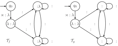
Figure 1 illustrates the distinction Definition 4 is unable to make.2 Function f is sequential, butgis not. Otherwise, they are identical. Whilef(bab) = bba,g(bab) = bbaa. With the original OSL
defini-tion, there is no way to refer to the output for input
babbeforethe final output string has been appended.
To deal with this problem we first define the prefix function associated to a subsequential function.
Definition 5 (Prefix function). Let f : Σ∗ → ∆∗
be a subsequential function. We define the prefix functionfp : Σ∗ → ∆∗ associated to f such that
fp(w) =lcp({f(wΣ∗)}).
2Here and in Figure 3, stateq
f is not shown. Non-initial
states are labeled q : u with q being the state’s name and (q,n, u, qf)∈δ.
Tf
q0
λ:λ !:λ
a:λ a:a
a:a
b:λ b:b
b:b b:a
a:b
q0
Tg
λ:λ !:λ
a:a a:a
a:a
b:b b:b
b:b b:a
a:b
[image:5.612.322.528.58.139.2]1
Figure 1: Two DSFST recognizing functions f and g.
Except for their final transitions,TfandTgare identical.
Remark 2. If T is an onward DSFST for f, then
∀w∈Σ∗,fp(w) =u⇐⇒ ∃q,(q0,ow, u, q)∈δ∗. Remark 3. Iff is sequential thenf =fp.
We can now revise the definition of OSL functions.
Definition 6 (Output Strictly Local Function (re-vised)). We say that a subsequential function f is
k-OSL if for allw1, w2 inΣ∗,Suffk−1(fp(w1)) =
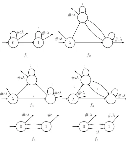
Suffk−1(fp(w2))⇒tailsf(w1) =tailsf(w2). Chandlee et al. (2014) provide several theorems which relate ISL functions, OSL functions (defined as in Definition 4), and SL stringsets. Here we ex-plain why those results still hold with Definition 6. The proofs for those results depend on the six func-tions (fi,1 ≤ i ≤ 6) reproduced here in Figure 2.
The transducers shown there are not DSFSTs but traditional subsequential transducers; readers are re-ferred to Chandlee et al. (2014) for formal defini-tions. With the exception off5, these functions are clearly sequential since each state outputs λ on n
(shown as#in Figure 2). The transducer forf5 is not onward, but an onward, sequential version of this transducer recognizing exactly the same function is obtained by suffixinga(which is thelcpof the
out-puts of state 1) onto the output of state 1’s incoming transition. Thus,f5is also sequential. By Remark 3 then, Theorems 4, 5, 6, and 7 of that paper still hold under Definition 6.
5 Automata characterization
First we show, for any non-initial state of any canon-ical transducer recognizing an OSL function, that if reading a letteraimplies writingλ, then this corre-sponds to a self-loop. So writing the empty string never causes a change of state (except fromq0).
Lemma 2. For any OSL functionfwhose canonical
0 a 1
#:λ #:λ
b,c a,b:a,c
f1
a
b
λ
b a a
b #:λ
#:λ
#:λ
a:b
b
f2
1 a
b
λ
a a
b,c:b #:λ
#:λ
#:λ
a,b:a,c:a
b,c:b
f3
a
b
λ
b a:aa a:aa
b #:λ
#:λ
#:λ
a:aa
b
f4
1
0 1
a
#:λ #:a
a
f5
1 0
a
a:λ
#:λ
#:λ
f6
[image:6.612.82.295.57.297.2]1
Figure 2: Examples used in proofs of Theorems 4 to 7 of Chandlee et al. (2014, see Figure 2).
that(q, a, λ, q0)∈δCthenq0 =q.
Proof. Consider w and u such that
(q0,ow, u, q) ∈ δC∗ and suppose(q, a, λ, q0) ∈ δC.
Then fp(w) = fp(wa) which implies
Suffk−1(fp(w)) = Suffk−1(fp(wa)). As f
is k-OSL, tailsf(w) = tailsf(wa). As TC
is canonical the non-initial and non-final states correspond to unique tail-equivalence classes, and two distinct states correspond to two different classes. Thereforeq0 =q.
Next we definek-OSL transducers.
Definition 7 (k-OSL transducer). An onward
DS-FSTT =hQ, q0, qf,Σ,∆, δiisk-OSL if
1. Q=S∪ {q0, qf}withS⊆∆≤k−1
2. (∀u ∈ ∆∗)(q0,o, u, q0) ∈ δ =⇒ q0 =
Suffk−1(u)
3. (∀q ∈Q\{q0},∀a∈Σ,∀u∈∆∗)
(q, a, u, q0)∈δ =⇒q0 =Suffk−1(qu).
Next we show thatk-OSL functions and functions
represented byk-OSL DSFSTs exactly correspond.
Lemma 3(extended transition function). Let T =
hQ, q0, qf,Σ,∆, δibe ak-OSL DSFST. We have
(q0,ow, u, q)∈δ∗ =⇒q=Suffk−1(u)
Proof. By recursion on the size ofw∈Σ∗. The
ini-tial case is valid for|w|= 0since if(q0,o, u, q) ∈
δ∗ then (q0,o, u, q) ∈ δ. By Definition 7, q =
Suffk−1(u). Suppose now that the lemma holds for
inputs of sizen 6= 0. Let wbe of sizensuch that (q0,ow, u, q) ∈ δ∗ and suppose (q, a, v, q0) ∈ δ (i.e., (q0,owa, uv, q0) ∈ δ∗). By recursion, we know that q = Suffk−1(u). By Definition 7, q0 = Suffk−1(qv) = Suffk−1(Suffk−1(u)v) =
Suffk−1(uv)(by Remark 1).
Lemma 4. Anyk-OSL DSFST corresponds to ak
-OSL function.
Proof. Let T = hQ, q0, qf,Σ,∆, δi be a k
-OSL DSFST computing f and let w1, w2 ∈ Σ∗ such that Suffk−1(fp(w
1)) = Suffk−1(fp(w2)). Since T is onward, by Remark 2 there exists
q, q0 ∈ Q such that(q0,ow1, fp(w1), q) ∈ δ∗ and
(q0,ow2, fp(w2), q0) ∈ δ∗. By Lemma 3, q =
Suffk−1(fp(w1)) =Suffk−1(fp(w2)) = q0which impliestailsf(w1) =tailsf(w2). Thereforefis ak-OSL function.
We now need to show that everyk-OSL function
can be represented by a k-OSL DSFST. An issue
here is that one cannot work fromTC since its states
are defined in terms of its tails, which themselves are defined in terms ofinputstrings, not output strings. Hence, the proof below is constructive.
Theorem 3. Letf be ak-OSL function. The DSFST
T defined as followed computesf:
• Q=S∪ {q0, qf}withS ⊆∆≤k−1
• (q0,o, u,Suffk−1(u))∈δ⇐⇒u=fp(λ) • a ∈ Σ, (q, a, u,Suffk−1(qu)) ∈ δ, ⇐⇒
(∃w)Suffk−1(fp(w)) = q∧fp(wa) = vqu
withv=fp(w)·q−1,
• (q,n, u, qf) ∈ δ ⇐⇒ u =fp(wq)−1·f(wq),
where wq = min{w | ∃u,(q0,ow, u, q) ∈
δ∗}.
The diagram below helps express pictorially how the transitions are organized per the second and third bullets above. The input is written above the arrows, and the output written below.
q0 −−−−−−→ow
fp(w)=vq q
a
Note thatT is ak-OSL SFST. To prove this result,
we first show the following lemma:
Lemma 5. LetT be the transducer defined in The-orem 3. We have:
(q0,ow, u, q)∈δ∗ ⇐⇒fp(w) =u
Proof. (⇒) By recursion on the length ofw.
Sup-pose (q0,ow, u, q) ∈ δ∗ and |w| = 0. Then
(q0,o, u, q)∈ δ; by construction,q =Suffk−1(u) andfp(λ) =uwhich validates the initial case.
Suppose the result holds forwof sizenand pick
such aw. Suppose then that(q0,owa, u, q) ∈ δ∗. By definition ofδ∗, there exists u1, u2, q0 such that
u=u1u2,(q0,ow, u1, q0)∈δ∗ and(q0, a, u2, q)∈
δ. We have fp(w) = u
1 (by recursion) and thus
q0 =Suffk−1(fp(w))(by Lemma 3).
By construction of T, q = Suffk−1(q0u2) and thus fp(wa) = vq0u
2 with v =
fp(w) ·Suffk−1(fp(w))−1. Therefore fp(wa) = vq0u2 = fp(w) · Suffk−1(fp(w))−1q0u2 =
fp(w) ·Suffk−1(fp(w))−1Suffk−1(fp(w))u
2 =
fp(w)u2 =u1u2 =u.
(⇐) By recursion on the length of w. If |w| = 0, then fp(λ) = u. By construction of T, (q0,o, u,Suffk−1(u)) ∈ δ, which validates the base case.
Now fix n > 0 and suppose the result holds
for all w of size n. Pick such a w and let
fp(wa) = u. As f is subsequential, there
ex-ists u1 such that fp(w) = u1. By recursion, there exists q such that (q0,ow, u1, q) ∈ δ∗. By Lemma 3, q = Suffk−1(u1) = Suffk−1(fp(w)). By definition fp(wa) = u1u−11 · u, which equals u1 · Suffk−1(u1)−1Suffk−1(u1)u−11 · u. Hence fp(wa) = vqu0, with u0 = u−11 · u
and v = u1 · Suffk−1(u1)−1, which equals
fp(w)·Suffk−1(fp(w))−1. Thus, by construction
(q, a, u0,Suffk−1(qu0))∈δ. Sinceu1u0 =u1u−11·
u=u,(q0,owa, u,Suffk−1(qu0))∈δ∗. We can now prove Theorem 3.
Proof. Let T be the transducer defined in Theo-rem 3. We show that∀w∈Σ∗,
(w, u)∈R(T)⇐⇒f(w) =u.
By definition of R(T), we know that (q0,own, u, qf) ∈ δ∗. By definition of δ∗,
q0
λ:λ
C:λ
˜ V:λ
V:λ
N:λ !:λ C:C
V:V N:N
V: ˜V C:C
V:V
C:C
N:N N:N
C:C
N:N N:N
V: ˜V
V:V C:C
[image:7.612.324.526.67.207.2]1
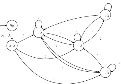
Figure 3: A 2-OSL DSFST that models Johore Malay nasal spreading.Σ={C, N, V}and∆={C, N, V, ˜V}.
there exists u1, u2 ∈ ∆∗ and q ∈ Q\{q0, qf}
such that (q0,ow, u1, q) ∈ δ∗, (q,n, u2, qf) ∈ δ,
and u = u1u2. By Lemma 5 we know that
fp(w) = u1. By construction of the DS-FST, we have u2 = fp(wq)−1 · f(wq) where wq = min{w0 | ∃u,(q0,ow0, u0, q) ∈ δ∗}. Therefore(wq, u0u2)∈R(T). Again, by Lemma 5,
fp(w
q) = u0 and so u0u2 = fp(wq)u2 =
fp(wq)fp(wq)−1·f(wq) =f(wq).
We have Suffk−1(u1) = Suffk−1(fp(wq)) = Suffk−1(fp(w)). As f is k-OSL, we know tailsf(wq) = tailsf(w), which implies that (λ, fp(w
q)−1·f(wq))∈tailsf(w). Thusf(w) = fp(w)fp(wq)−1·f(wq) =u1u2 =u.
Figure 3 presents a 2-OSL transducer that mod-els the nasal spreading example from§2. Note C=
obstruent, V=vowels and glides, ˜V=nasalized V,
and N=nasal consonant.
6 Learning OSL functions
6.1 Learning criterion
We adopt the identification in the limit learning paradigm (Gold, 1967), with polynomial bounds on time and data (de la Higuera, 1997). The underlying idea of the paradigm is that if the data available to the algorithm does not contain enough information to distinguish the target from other potential targets, then it is impossible to learn.
We first need to define the following notions. A class T of functions is represented by a class R
and there is a total and surjective naming function L : R → T such thatL(r) = tif and only if for
all w ∈ pre image(t), r(w) = t(w), wherer(w)
is the output of representationron the inputw. We
observe that the class ofk-OSL functions can be
rep-resented by the class ofk-OSL DSFSTs.
Definition 8. Let T be a class of functions repre-sented by some classRof representations.
1. AsampleSfor a functiont∈Tis a finite set of
data consistent witht, that is to say(w, v)∈S
ifft(w) =v. The size of a sampleSis the sum
of the length of the strings it is composed of: |S|=P(w,v)∈S|w|+|v|.
2. A (T,R)-learning algorithm A is a program that takes as input a sample for a functiont∈T
and outputs a representation fromR.
The paradigm relies on the notion of characteristic sample, adapted here for functions:
Definition 9(Characteristic sample). For a(T,R)
-learning algorithmA, a sample CS is a
character-istic sample of a function t ∈ T if for all samples
S fortit is the case thatCS ⊆S andAreturns a representationrsuch thatL(r) =t.
This definition is the one used in the proof of the OSTIA algorithm. The learning paradigm can now be defined as follows.
Definition 10 (Identification in polynomial time and data). A class Tof functions is identifiable in polynomial time and data if there exists a (T,R)
-learning algorithmAand two polynomialsp()and q()such that:
1. For any sampleSof sizemfort∈T,Areturns a hypothesisr ∈RinO(p(m))time.
2. For each representationr ∈ Rof size n, with
t = L(r), there exists a characteristic sample
oftforAof size at mostO(q(n)).
6.2 Learning algorithm
We show here that Algorithm 1 learns the OSL func-tions under the criterion introduced. We call this the Output Strictly Local Function Inference Algorithm (OSLFIA). We assumeΣ,∆, andkare fixed and not part of the input to the learning problem.
Essentially, the algorithm computes a breadth-first search through the states that are reachable
Data: SampleS⊂ {o}Σ∗{n} ×∆∗and k∈N
Letq0, qf be states with{q0, qf} ∩∆≤k−1=∅ s←lcp({y|(x, y)∈S});q←Suffk−1(s); smallest(q) =o;out(q) =s;
δ ← {(q0,o, s, q)};R← {q};C← {q0, qf};
whileR6=∅do
q ←f irst(R);s←smallest(q);
foralla∈Σin alphabetical orderdo
if∃(w, u)∈S,x∈Σ∗ s.t.w=sax
then
v←lcp({y| ∃x,(sax, y)∈S}); r←Suffk−1(qv);
δ←δ∪ {(q, a,out(q)−1·v, r)};
ifr /∈R∪Cthen R←R∪ {r}; smallest(r)←sa; out(r)←v;
if∃u,(s, u)∈Sthen
δ ←δ∪ {(q,n,out(q)−1·u, qf)} R←R\ {q};
C ←C∪ {q};
returnhC, q0, qf,Σ,∆, δi;
Algorithm 1:OSLFIA
given the learning sample: the set C contains the
states already checked whileR is a queue made of
the states that are reachable but have not been treated yet. Initially, the only transition leaving the initial state is writing thelcp of the output strings of the
sample and reaches the state corresponding to the
k−1suffix of this lcp. At each step of the main
loop, OSLFIA treats the first state that is in the queue
R and computes whenever possible the transitions
that leave that state. The outputs associated with each added transition are the longest common pre-fixes of the outputs associated with the smallest in-put prefix in the sample that allows the state to be reachable. We show that provided the algorithm is given a sufficient sample the transducer outputted by OSLFIA is onward and in fact ak-OSL transducer.
After adding transitions with input letters fromΣto a state, the transition to the final state is added, pro-vided it can be calculated.
6.3 Theoretical results
-OSL functions in polynomial time and data.
Lemma 6. For any input sample S, OSLFIA
pro-duces its output in time polynomial in the size ofS.
Proof. The main loop is used at most|∆|k−1which
is constant since both ∆ and k are fixed for any
learning sample. The smaller loop is executed|Σ| times. At each execution: the first conditional can be tested in time linear inn, wheren=P(w,u)∈S|w|;
the computation of thelcpcan be done innmsteps
wherem=max{|u|: (w, u) ∈S}with an appro-priate data structure (for instance a prefix tree); com-puting the suffix requires at mostmsteps. The
sec-ond csec-onditional can be tested in at mostcard(S)·m
steps; the computation of the final transitions can be done in less thanmsteps; all the other instructions can be done in constant time. The overall computa-tion time is thusO(|∆|k−1|Σ|(n+nm+card(S)· m+ 2m)) =O(n+m(n+card(S))which is poly-nomial (in fact bounded by a quadratic function) in the size of the learning sample.
Next we show that for each k-OSL function f,
there is a finite kernel of data consistent with f (a
‘seed’) that is a characteristic sample for OSLFIA.
Definition 11 (A OSLFIA seed). Given a k-OSL
transducer hQ, q0, qf,Σ,∆, δi computing a k-OSL
functionf, a sampleSis a OSLFIAseedforf if
• For all q ∈ Q such that ∃v ∈ ∆∗ (q,n, v, qf) ∈ δ,(owqn, f(wq)) ∈ S, where wq = min{w| ∃u,(q0,ow, u, q)∈δ∗} • For all (q, a, u, q0) ∈ δ with q0 6= qf and
a∈ {o}∪Σ, for allb∈Σsuch that there exists (q0, b, u0, q00) ∈δ, there exists(own, f(w))∈
S and x ∈ Σ∗ such that w = wqabx and f(w)is defined. Also, if there existsvsuch that (q0,n, v, qf)∈δthen(owqan, f(wqa))∈S.
In what follows, we set T =
hQ, q0, qf,Σ,∆, δi be the target k-OSL
transducer, f the function it computes, and T =hQ, q0, qf,Σ,∆, δibe the transducer OSLFIA
constructs on a sample that contains a seed.
Lemma 7. If a learning sample S contains a seed
then(q0,ow, u, r)∈δ∗ ⇐⇒(q0,ow, u, r)∈δ∗. Proof. (⇒). By induction on the length of w. If
|w|= 0then(q0,o, u, r) ∈δand sou =lcp({y |
(x, y) ∈ S})andr = Suffk−1(u) (initial steps of
the algorithm). As S is a seed there is an element (obxn, f(bx))∈Sfor allb∈Σand(on, f(λ))∈
S if λ ∈ pre image(f), which implies that u = lcp(f(λΣ∗)). As the target is onward, we have (q0,o,lcp(f(λΣ∗)), r0) ∈ δ and since it is a
k-OSL DSFST r0 = Suffk−1(lcp(f(λΣ∗))) = Suffk−1(u) =r.
Suppose the lemma is true for strings of length less than or equal to n. We refer to this as
the first Inductive Hypothesis (IH1). Let wa be
of size n + 1 such that (q0,owa, u, r) ∈ δ∗. By definition of δ∗, there exist u1, u2, q such that
(q0,ow, u1, q) ∈ δ∗, (q, a, u2, r) ∈ δ, and u =
u1u2. By IH1 (q0,ow, u1, q) ∈ δ∗. We want to show(q0,owa, u, r)∈δ∗(i.e.,(q, a, u2, r)∈δ).
First we show that IH1 also implies that s = smallest(q) such thats = owq. Since the
algo-rithm searches breadth-first, sis the smallest input
that reachesq inT. If owqsthen ∃q0 6=q such
that(q0,owq, u0, q0) ∈ δ∗ becauseowq is a prefix
of an input string of the sampleS(sinceScontains
a seed). Since owqsand|s| ≤ n, by IH1 then (q0,owq, u0, q0) ∈δ∗ which impliesq =q0 which
contradicts the supposition thatowqs. Ifsowq,
then again since (q0,os, u0, q) ∈ δ∗ then by IH1
(q0,os, u0, q)∈δ∗. This contradicts the definition ofwq. Therefores=owq.
Next we show that IH1 impliesfp(w
q) =out(q).
By construction of the seed,(owqn, f(wq))∈Sif
∃v(q,n, v, qf)∈δand(owqaw0n, f(wqaw0))∈
Sfor all transitions(q, a, x, q0)leavingqinT. As
the target is onward,lcp({x|(q, σ, x, q0)∈δ, σ∈ Σ∪ {n}} =λ(Lemma 1). This impliesout(q) = lcp({y | ∃a∈Σ, x∈Σ∗{n},(osax, y)∈S}) = lcp({y | ∃a ∈ Σ, x ∈ Σ∗{n},(owqax, y) ∈ S}) =lcp({f(wqΣ∗)}) =fp(wq).
Recalling that (q, a, u2, r) ∈ δ, we now char-acterize u2 to help establish (q, a, u2, r) ∈ δ. By construction of a seed, there exist elements
(owqabxn, f(wqabx))inS for all possibleb ∈ Σ
and an element(owqan, f(wqa)) ∈ S if f(wqa)
is defined. By the onwardness of the target, this implies that v = lcp({y | ∃b, x,(osabxn, y) ∈ S} ∪ {f(sa)}) =lcp(f(saΣ∗)) = fp(sa).
There-fore u2 = out(q)−1 ·v = fp(s)−1 · fp(sa) =
fp(wq)−1·fp(wqa).
of the proof. As the target is OSL, we have
(q0,owqa, fp(wqa), r0) ∈ δ∗ (Lemma 3). The fact that (q0,owq, fp(wq), q) ∈ δ∗ by IH1 and
the fact the target is OSL implies(q, a, fp(wq)−1 · fp(w
qa), r0) = (q, a,out(q)−1 ·s, r0) ∈ δ. As T isk-OSL,r0 = Suffk−1(qout(q)−1·s)which is r by construction of the transition in the
algo-rithm. Therefore, as (q0,ow, u1, q) ∈ δ∗ by IH1, we have (q0,owa, u1out(q)−1 · s, r) =
(q0,owa, u1u2, r) = (q0,owa, u, r)∈δ∗ (⇐). This is also by induction on the length of w. If |w| = 0, as T is onward we have
lcp(outputs(q0)) = lcp(f(Σ∗)) (Lemma 1)
and thus (q0,o,lcp(f(Σ∗)), r) ∈ δ with r =
Suffk−1(lcp(f(Σ∗))) as T is k-OSL. By con-struction of the seed, there is at least one ele-ment in S using each transition leaving r. As lcp(outputs(r)) = λ (Lemma 1), this implies
lcp({y | (x, y) ∈ S}) = lcp(f(Σ∗)). Therefore (q0,o,lcp(f(Σ∗)), r)∈δ.
Suppose the lemma is true for all strings up to length n. We refer to this as the second Inductive
Hypothesis (IH2). Pick wa of length n + 1 such
that (q0,owa, u, r) ∈ δ∗. By definition of δ∗,
q, u1, u2 exist such that (q0,ow, u1, q) ∈ δ∗ and
(q, a, u2, r) ∈ δ, with u1u2 = u. By IH2, we have (q0,ow, u1, q),(q0,owq, u01, q) ∈ δ∗ (since
wqw). We want to show(q, a, u2, r)∈δ.
We first show that s = smallest(q) = owq.
Suppose sowq. By construction of the SFST s
is a prefix of an element of S which means there
exists q0 such that (q0, s, fp(s), q0) ∈ δ∗. But by IH2, this implies thatq0 = q and the definition of wqcontradictssowq. Suppose now thatowqs.
By the construction of the seed,owqis a prefix of an
element of the sample, which implies it is considered by the algorithm. As(q0,owq, u01, q) ∈ δ∗ by IH2,
owqis a smaller prefix thansthat reaches the same
state which is impossible as sis the earliest prefix that makes the stateq reachable. Thereforeowq = s and thus the transition from state q reading a is
created whens=owq.
Next we show that fp(wq) = out(q). By
construction of the seed, there is an element
(owqaw0n, f(wqaw0)) ∈ S for all transitions (q, a, x, q0) ∈ δ leaving q and(owqn, f(wq)) ∈ S if ∃v, (q,n, v, qf) ∈ δ. As the target is onward, lcp({x | (q, σ, x, q) ∈ δ∗, σ ∈ Σ ∪
n} = λ (Lemma 1). This implies out(q) = lcp({y | ∃a, x,(sax, y) ∈ S}) = lcp({y |
∃a, x,(wqax, y) ∈ S}) = lcp(f(wqΣ∗)) = fp(wq) =fp(s).
Now let v = lcp({y | ∃b, x,(sabx, y) ∈ S}).
Sinces=owq,(q0,owqa, v, r)∈δ∗since, as
be-fore, the onwardness of the target implies thelcpof
the output written fromrisλ. This is because each
possible output from r is in S (because it is in the seed according to the second item of Definition 11). Consequentlyv=fp(wqa) =fp(sa).
Together these results imply thatu2 =fp(wq)−1· fp(wqa) =fp(s)−1·fp(sa) =out(q)−1·v.
As the target is ak-OSL transducer (and thus
de-terministic)Suffk−1(qu2) =r. Therefore the tran-sition(q, a,out(q)−1·v, r)that is added toδis the
same as the transition(q, a, u2, r)inδ. This implies
(q0,owa, u, r)∈δ∗ and proves the lemma.
Lemma 8. Any seed for the OSL Learner is a char-acteristic sample for this algorithm.
Proof. A corollary of Lemma 7 is that if a seed is contained in a learning sample we have
(q0,ow, u, q)∈ δ∗ ⇐⇒ fp(w) =u(Lemma 3) as the target transducer isk-OSL. For all statesqwhere
∃v, (q,n, v, qf) ∈ δ, we have (owqn, f(wq))
in the seed, which implies the algorithm will add
(q,n, fp(wq)−1 ·f(wq), qf) to δ which is exactly
the output function of the target. As every state is treated only once, this holds for any learning set containing a seed. Therefore, from any super-set of a seed, for anyw, the function computed by
the outputted transducer of Algorithm 1 is equal to
fp(w)fp(w)−1·f(w) =f(w).
Observe that OSLFIA is designed to work with seeds, which contains minimalstrings. We believe both the seed and algorithm can be adjusted to relax this requirement, though this is left for future work.
Lemma 9. Given anyk-OSL transducer T, there
exists a seed for the OSL learner that is of size poly-nomial in the size ofT.
Proof. LetT =hQ
, q0, qfΣ,∆, δ,i. There are at most card(Q) pairs (owqn, f(wq)) in a seed
and|f(wq)| ≤P(q,σ,u,q0)∈δ|u|. We denote bym
this last quantity and note thatm =O(|T|).
For the elements of the second item of Def-inition 11 we restrict ourselves without loss of generality to pairs(owqabw0n, f(wqabw0))where w0 = min{x : f(wqabx)is defined}. We
have |w0| ≤ card(Q) and |f(wqabw0)| is in
O(card(Q)m). There are at most |Σ| pairs
(owqabw0n, f(wqabw0)) for a given transition (q, a, u, q0) which implies that the overall bound
on the number of such pairs is in O(|Σ|card(δ)). The overall length of the elements in the seed that fulfill the second item of the definition is in O(card(Q)(card(Q) +m+|Σ|card(δ)m)).
The size of the seed studied in this proof is thus in O((m+|Q|)(|Q|+|Σ|card(δ))which is poly-nomial (in fact quadratic) in the size of the target transducer.
Theorem 4. OSLFIA identifies thek-OSL functions in polynomial time and data.
Proof. Immediate from Lemmas 6, 7, 8, and 9.
We conclude this section by comparing this result to other subsequential function-learning algorithms. OSTIA (Oncina et al., 1993) is a state-merging algorithm which can identify the class of total sub-sequential functions in cubic time. (Partial subse-quential functions cannot be learned exactly; for a partial function, OSTIA will learn some superset of it.) k-OSL functions include both partial and total
functions, so the classes exactly learnable by OSTIA and OSLFIA are, strictly speaking, incomparable.
SOSFIA (Jardine et al., 2014) identifies sub-classes of subsequential functions in linear time and data. These subclasses are determined by fixing the structure of a transducer in advance. For every in-put string, SOSFIA knows exactly which state in the transducer is reached. The sole carrier of informa-tion regarding reached states is the input string. But fork-OSL functions, the output strings carry the
in-formation about the states reached. As the theorems demonstrate, the destination of a transition is only determined by the output of the transition. Thus no class learned by SOSFIA contains anyk-OSL class.
OSTIA-D (OSTIA-R) (Oncina and Var`o, 1996; Castellanos et al., 1998) identify a class of subse-quential functions with a given domainD(rangeR)
in at least cubic time because it adds steps to OSTIA to prevent merging states that would result in a trans-ducer whose domain (range) is not compatible with
D(R). OSTIA-D cannot representk-OSL functions
for the same reasons SOSFIA cannot: domain in-formation is about input strings, not output strings. On the other hand, the range of a k-OSL function
is ak-OSL stringset which can be represented with
a single acceptor, and thus OSL functions may be learned by OSTIA-R. However, OSLFIA is more ef-ficient both in time and data.3
To sum up, OSLFIA is the most efficient algo-rithm for learningk-OSL functions.
7 Phonology
The example of Johore Malay nasal spreading given in§2 is an example of progressive spreading, since it proceeds from a triggering segment (the nasal) to vowels and glides that follow it. There also exist regressivespreading processes, in which the trigger follows the target(s). An example from the M`ob`a di-alect of Yoruba (Aj´ıb´oy`e, 2001; Aj´ıb´oy`e and Pulley-blank, 2008; Walker, 2014) is shown in (2). An un-derlying nasalized vowel spreads its nasality to pre-ceding oral vowels and glides.
(2) /uj˜i/7→[˜u˜j˜i], ‘praise(n.)’
The difference between progressive and regressive spreading corresponds to reading the input from left-to-right or right-to-left, respectively (Heinz and Lai, 2013). Regressive spreading cannot be modeled with OSL in a left-to-right fashion, because the out-put of the preceding vowels and glides depends on the presence or absence of a following nasal that could be an unbounded number of segments away. By reading from right-to-left, that nasal trigger will always be read before the target(s), making it akin to progressive spreading. Thus there are two overlap-ping but non-identical classes, which we call left(-to-right) OSL and right(-to-left) OSL.
There are other types of phonological maps that are neither ISL nor OSL. Consider the optional pro-cess of French@-deletion shown in (3) (Dell, 1973; Dell, 1980; Dell, 1985; Noske, 1993).
(3) @→ ∅/ VC CV
At issue is how this rule applies. There are two licit pronunciations of /ty d@v@nE/ ‘you became’ which are [ty dv@nE] and [ty d@vnE]. The form *[ty dvnE] is considered ungrammatical. As Ka-plan and Kay (1994) explain, these outputs can be understood as the rule in (3) applying left-to-right ([ty dv@nE]), right-to-left ([ty dv@nE]) or simultane-ously (*[ty dvnE]). What matters is whether the left and right contexts of the rule match theinputor out-putstring: if both match the input it is simultaneous application, and if one side matches the input and the other the output it is left-to-right or right-to-left. ISL functions always match contexts against the input and therefore they cannot model@-deletion. In this respect, ISL functions model simultaneous rule application. But there is also a problem with mod-eling the process as OSL, which is what to output when the@that will be deleted is read. Consider the input VC@CV. When the DSFST reads the@, it can-not decide what to output, because whether or can-not that@is deleted depends on whether or not the next two symbols in the input are CV. But since the DS-FST is deterministic, it must make a decision at this point. It could postpone the decision and outputλ.
But that would require it to loop at the current state (Lemma 2), which in turn means it cannot distin-guish VC@CV from VC@@@CV, a significant problem since only the former meets the context for deletion. Thus the range of phonological processes that can be modeled with OSL functions is limited to those with one-sided contexts (e.g., either C or D, the former being left OSL and the latter right OSL). In such cases the entire triggering context will be read before the potential target, so there is never a need to delay the decision about what to output. To summa-rize, phonological rules that apply simultaneously are ISL, and phonological rules with one-sided con-texts that apply left-to-right or right-to-left are OSL. In addition to iterative rules with two-sided con-texts, long-distance processes like vowel harmony and consonant agreement and dissimilation are also excluded from the current analysis. While such process have been shown to be subsequential and therefore subregular (see Gainor et al. (2012; Luo (2014; Payne (2013; Heinz and Lai (2013)) they are neither ISL nor OSL because the target and
trigger-ing context are not within a fixed window of length
k in either the input or output. An example is the
long-distance nasal assimilation process in Kikongo (Rose and Walker, 2004), as in (4).
(4) /tu+nik+idi/7→[tunikini] ‘we ground’ In Kikongo, the alveolar stop in the suffix /-idi/ sur-faces as a nasal when joined to a stem containing a nasal. Since stem nasals appear to occur arbitrarily far from the suffix, there is noksuch that the target
/d/ and the trigger /n/ are within a window of sizek.
Thus the process is neither ISL nor OSL.
8 Future Work
Processes like French@-deletion that have two-sided contexts, with one being on the output side, sug-gest a class that combines the ISL and OSL prop-erties. We are tentatively calling this class ‘Input-Output SL’ and are currently working on its prop-erties, FST characterization, and learning algorithm. For long-distance processes, we expect other func-tional subclasses will strongly characterize these. SL stringsets are just one region of the Subregular Hierarchy (Rogers and Pullum, 2011; Rogers et al., 2013), so we expect functional counterparts of the other regions can be defined. Some of these other regions model long-distance phonotactics (Heinz, 2007; Heinz, 2010; Rogers et al., 2010), so their functional counterparts may prove equally useful for modeling and learning long-distance phonology.
9 Conclusion
We have defined a subregular class of func-tions called the OSL funcfunc-tions and provided both language-theoretic and automata-theoretic charac-terizations. The structure of this class is sufficient to allow anyk-OSL function to be efficiently learned
from positive data. It was shown that the OSL functions—unlike the ISL functions—can model lo-cal iterative spreading processes. Future work will aim to combine the results for both ISL and OSL to model iterative processes with two-sided contexts.
Acknowledgments
References
Ol´adi´ıp`o Aj´ıb´oy`e and Douglas Pulleyblank. 2008. M`ob`a nasal harmony. Ms., University of Lagos and Univer-sity of British Columbia.
Ol´adi´ıp`o Aj´ıb´oy`e. 2001. Nasalization in M`ob`a. In Suny-oung Oh, Naomi Sawai, Kayono Shiobara, and Rachel Wojdak, editors, Proceedings of the Northwest Lin-guistics Conference, pages 1–18. University of British Columbia Working Papers in Linguistics 8. Vancou-ver: University of British Columbia, Department of Linguistics.
William Bennett. 2013. Dissimilation, Consonant Har-mony, and Surface Correspondence. Ph.D. thesis, Rut-gers.
Antonio Castellanos, Enrique Vidal, Miguel A. Var´o, and Jos´e Oncina. 1998. Language understanding and sub-sequential transducer learning. Computer Speech and Language, 12:193–228.
Jane Chandlee and Jeffrey Heinz. 2012. Bounded copy-ing is subsequential: Implications for metathesis and reduplication. In Proceedings of the 12th Meeting of the ACL Special Interest Group on Computational Morphology and Phonology, pages 42–51, Montreal, Canada, June. Association for Computational Linguis-tics.
Jane Chandlee and Jeffrey Heinz. to appear. Strictly lo-cal phonologilo-cal processes. Linguistic Inquiry,. under revision.
Jane Chandlee, Angeliki Athanasopoulou, and Jeffrey Heinz. 2012. Evidence for classifying metathesis pat-terns as subsequential. InThe Proceedings of the 29th West Coast Conference on Formal Linguistics, pages 303–309. Cascadilla Press.
Jane Chandlee, R´emi Eyraud, and Jeffrey Heinz. 2014. Learning strictly local subsequential functions. Trans-actions of the Association for Computational Linguis-tics, 2:491–503, November.
Jane Chandlee. 2014. Strictly Local Phonological Pro-cesses. Ph.D. thesis, The University of Delaware. Noam Chomsky and Morris Halle. 1968. The Sound
Pattern of English. New York: Harper & Row. Colin de la Higuera. 1997. Characteristic sets for
polynomial grammatical inference. Machine Learning Journal, 27:125–138.
Franc¸ois Dell. 1973. Les r´egles et les sons. Paris: Her-mann.
Franc¸ois Dell. 1980. Generative phonology and French phonology. Cambridge: Cambridge University Press. Franc¸ois Dell. 1985. Les r´egles et les sons. Paris:
Her-mann, 2 edition.
Jason Eisner. 2003. Simpler and more general minimiza-tion for weighted finite-state automata. InProceedings
of the Joint Meeting of the Human Language Technol-ogy Conference and the North American Chapter of the Association for Computational Linguistics (HLT-NAACL 2003), pages 64–71.
Robert Frank and Giorgo Satta. 1998. Optimality Theory and the generative complexity of constraint violability.
Computational Linguistics, 24(2):307–315.
Brian Gainor, Regine Lai, and Jeffrey Heinz. 2012. Computational characterizations of vowel harmony patterns and pathologies. In Jaehoon Choi, E. Alan Hogue, Jeffrey Punske, Deniz Tat, Jessamyn Schertz, and Alex Trueman, editors,WCCFL 29: Proceedings of the 29th West Coast Conference on Formal Linguis-tics, pages 63–71, Somerville, MA. Cascadilla. E.Mark Gold. 1967. Language identification in the limit.
Information and Control, 10:447–474.
Thomas Graf. 2010. Logics of phonological reasoning. Master’s thesis, University of California, Los Angeles. Gunnar Hansson. 2010. Consonant Harmony: Long-Distance Interaction in Phonology. Number 145 in University of California Publications in Linguistics. University of California Press, Berkeley, CA. Avail-able on-line (free) at eScholarship.org.
Jeffrey Heinz and Regine Lai. 2013. Vowel harmony and subsequentiality. In Andras Kornai and Marco Kuhlmann, editors, Proceedings of the 13th Meeting on the Mathematics of Language (MoL 13), pages 52– 63, Sofia, Bulgaria.
Jeffrey Heinz. 2007. The Inductive Learning of Phono-tactic Patterns. Ph.D. thesis, University of California, Los Angeles.
Jeffrey Heinz. 2009. On the role of locality in learning stress patterns. Phonology, 26(2):303–351.
Jeffrey Heinz. 2010. Learning long-distance phonotac-tics. Linguistic Inquiry, 41(4):623–661.
Adam Jardine, Jane Chandlee, R´emi Eyraud, and Jef-frey Heinz. 2014. Very efficient learning of struc-tured classes of subsequential functions from positive data. In Alexander Clark, Makoto Kanazawa, and Ryo Yoshinaka, editors, Proceedings of the Twelfth Inter-national Conference on Grammatical Inference (ICGI 2014), volume 34, pages 94–108. JMLR: Workshop and Conference Proceedings, September.
Adam Jardine. 2014. Computationally, tone is different. Under review with Phonology.
C. Douglas Johnson. 1972.Formal Aspects of Phonolog-ical Description. The Hague: Mouton.
Ronald Kaplan and Martin Kay. 1994. Regular models of phonological rule systems. Computational Linguis-tics, 20(3):331–378.
Huan Luo. 2014. Long-distance consonant harmony and subsequantiality. Qualifying paper for the University of Delaware’s Linguistics PhD Progam.
Robert McNaughton and Seymour Papert. 1971.
Counter-Free Automata. MIT Press.
Mehryar Mohri. 1997. Finite-state transducers in lan-guage and speech processing.Computational Linguis-tics, 23(2):269–311.
Andrew Nevins. 2010.Locality in Vowel Harmony. MIT Press.
Roland Noske. 1993. A theory of syllabification and seg-mental alternation. Niemeyer, T¨ubingen.
David Odden. 2014. Introducing Phonology. Cam-bridge University Press, 2nd edition.
Jose Oncina and Pedro Garcia. 1991. Inductive learning of subsequential functions. Technical Report DSIC II-34, University Polit´ecnia de Valencia.
Jos´e Oncina and Miguel A. Var`o. 1996. Using do-main information during the learning of a subsequen-tial transducer. Lecture Notes in Artificial Intelligence, pages 313–325.
Jos´e Oncina, Pedro Garc´ıa, and Enrique Vidal. 1993. Learning subsequential transducers for pattern recog-nition tasks. IEEE Transactions on Pattern Analysis and Machine Intelligence, 15:448–458, May.
Farid M. Onn. 1980. Aspects of Malay Phonology and Morphology: A Generative Approach. Kuala Lumpur: Universiti Kebangsaan Malaysia.
Amanda Payne. 2013. Dissimilation as a subsequen-tial process. Qualifying paper for the University of Delaware’s Linguistics PhD Progam.
James Rogers and Geoffrey Pullum. 2011. Aural pattern recognition experiments and the subregular hierarchy.
Journal of Logic, Language and Information, 20:329– 342.
James Rogers, Jeffrey Heinz, Gil Bailey, Matt Edlefsen, Molly Visscher, David Wellcome, and Sean Wibel. 2010. On languages piecewise testable in the strict sense. In Christian Ebert, Gerhard J¨ager, and Jens Michaelis, editors,The Mathematics of Language, vol-ume 6149 of Lecture Notes in Artifical Intelligence, pages 255–265. Springer.
James Rogers, Jeffrey Heinz, Margaret Fero, Jeremy Hurst, Dakotah Lambert, and Sean Wibel. 2013. Cog-nitive and sub-regular complexity. In Glyn Morrill and Mark-Jan Nederhof, editors, Formal Grammar, volume 8036 of Lecture Notes in Computer Science, pages 90–108. Springer.
Sharon Rose and Rachel Walker. 2004. A typology of consonant agreement as correspondence. Language, 80:475–531.
Jaques Sakarovitch. 2009. Elements of Automata The-ory. Cambridge University Press. Translated by
Reuben Thomas from the 2003 edition published by Vuibert, Paris.
Keiichiro Suzuki. 1998. A Typological Investigation of Dissimilation. Ph.D. thesis, University of Arizona. Wolfgang Thomas. 1997. Languages, automata, and
logic. volume 3, chapter 7. Springer.
Rachel Walker. 2011. Vowel Patterns in Language. Cambridge: Cambridge University Press.
Rachel Walker. 2014. Nonlocal trigger-target relations.