Munich Personal RePEc Archive
Sovereign defaults, external debt and
real exchange rate dynamics
Asonuma, Tamon
International Monetary Fund
23 March 2014
Online at
https://mpra.ub.uni-muenchen.de/55133/
Sovereign Defaults, External Debt and Real Exchange Rate
Dynamics
Tamon Asonumay
March 23, 2014
Abstract
Emerging countries experience real exchange rate depreciations around defaults. In this paper, we examine this observed pattern empirically and through the lens of a dynamic stochastic general equilibrium model. The theoretical model explicitly incorporates bond issuances in local and
foreign currencies, and endogenous determination of real exchange rate and default risk. Our quantitative analysis, using the case of Argentina’s default in 2001, replicates the link between real exchange rate depreciation and default probability around defaults and moments of the real exchange rate that match the data. Prior to default, interactions of real exchange rate depreciation, originated from a sequence of low tradable goods shocks with the sovereign’s large share of foreign currency debt, trigger defaults. In post-default periods, the resulting output costs and loss of market access due to default lead to further real exchange rate depreciation.
.
JEL Classi…cation Codes: E43; F32; F34; G12
Key words: Sovereign defaults; External debt; Real exchange rate; Currency composition of debt;
The views expressed in this paper are those of the author and do not re‡ect any views of the International Monetary Fund. I thank Manuel Amador, Marianne Baxter, Nicola Borri, Matthieu Bussiere, Marcos Chamon, Bora C. Durdu, Douglas Gale, Francois Gourio, Simon Gilchrist, Juan C. Hatchondo, Laurence Kotliko¤, Alberto Martin, Leonardo Martinez, Akito Matsumoto, Kris Mitchener, Ugo Panizza, Romain Ranciere, Francisco Roch, Martin Schneider, Chris-tian Siegel, Cedric Tille, Christoph Trebesch, Adrien Verdelhan, and Mark Wright, as well as seminar participants at Bank of Japan, Birmingham Business School, Boston University, Exeter Business School, Halle Institute for Economic Research, IMF AFR, IMF ICD, IMF RES, Keio Univ, Osaka Univ, and University of Munich for comments and sug-gestions. Additional thanks go to Haitham Jendoubi for research assistance and Christina M. Gebel for proof reading. All remaining errors are my own.
1
Introduction
Emerging market economies experience real exchange rate depreciations around the default events. We …rst empirically examine this stylized fact. The theoretical part of the paper explores interactions between real exchange rate and default decision in a stochastic general equilibrium model featuring defaultable debt. Our quantitative analysis, using Argentina’s default episode in 2001, successfully explains the link between real exchange rate depreciation and default probability and also matches the relevant moments in the data.
In the empirical section, we present a new stylized fact on real exchange rate dynamics around sovereign defaults. For 18 sovereign debt default and restructuring episodes in 1998-2013, we …nd the empirical link between the real exchange rate depreciation and default risk (default decision): In the period prior default, the real exchange rate depreciation increases the burden of payments and ultimately triggers the default. In the post-default period, the country’s announcement of default, or restructuring, leads to further real exchange rate depreciation. Our results on cross-sectional analysis, using these episodes, also con…rm the observed link - a new contribution to the literature on sovereign defaults. Motivated by this stylized fact, we aim to answer the following two questions which are not explained in the literature: What drives real exchange rate depreciation leading to the country’s default decision in the pre-default period? What leads to further real exchange rate depreciation in the post-default period?
default decision of the sovereign.
Once the sovereign declares default, it su¤ers output costs associated with default and loses access to the markets. By achieving …nancial autarky, the sovereign opts to have higher consumption of traded goods, indicating lower marginal utility of consumption, which leads to higher prices of non-traded goods and a higher overall price level relative to that of foreign creditors. Thus, it results in a further depreciation of the real exchange rate. This mechanism drives the equilibrium depreciation of the real exchange rate around defaults, and it is a plausible explanation of the observed patterns in the data.
The model is calibrated to the case of Argentina’s default in 2001. Our quantitative exercise successfully replicates both business cycle and non-business-cycle moments that match with the data. Most importantly, our model generates real exchange rate moments consistent with what we observe in the Argentine data, particularly a higher average real exchange rate in the post-default periods than in the pre-default periods. The current model explains the observed real exchange rate dynamics around defaults.
We embed the real exchange rate dynamics and currency denomination of debt in a dynamic, sovereign debt model with endogenous default. This part of the model builds on the recent quan-titative analysis of sovereign debt such as Aguiar and Gopinath (2006), Arellano (2008), and Tomz and Wright (2007), all of which are based on the classical setup of Eaton and Gersovitz (1981). To account for the creditor’s willingness to avoid real exchange rate risks and demanding an excess risk premium as observed in the real world, we depart from the conventional risk-neutral investor assump-tion. Instead, we assume a "representative" risk-averse creditor who faces exogenous income shocks, as in Borri and Verdelhan (2009) and Lizarazo (2013). Our model also amends the tranditional debt issuance in domestic currency and considers that a sovereign issues external bonds in both local and foreign currencies, as observed in the data, extending a traditional assumption of domestic currency debt issuance.
is presented in Appendix A.
1.1 Literature Review
Our paper builds on some strands of existing literature. First, this paper is related to the literature of sovereign debt and defaults, which extends a classical model of Eaton and Gersovitz (1981) and applies quantitative analysis. Arellano (2008) and Aguiar and Gopinath (2006) explore the connection between endogenous default, interest rates and income ‡uctuations in a model of sovereign debt and generate empirical regularities in emerging markets. Arellano and Heathcote (2010) explore what determines credit limits and how these vary across exchange rate regimes in a sovereign debt model.1
Asonuma (2012), Benjamin and Wright (2009), Bi (2008), and Yue (2010) model debt renegotiation after defaults and explain observed evidence of debt restructurings. This paper di¤ers in that we mainly focus on interactions between default choices and real exchange rate dynamics.
The second grouping of literature deals with sovereign debt and risk-averse investors. Borri and Verdelhan (2009), Lizarazo (2013), and Presno and Puozo (2011) study the case of risk-averse lenders and show that risk aversion allows the model to generate spreads larger than default probabilities, as observed in emerging markets. Borri and Verdelhan (2009) consider risk aversion with external habit preference, whereas Lizarazo (2013) assumes decreasing absolute risk aversion (DARA). On the contrary, Presno and Puozo (2011) introduce fears about model misspeci…cation for the lenders. What distinguishes this current paper with these studies is that we incorporate real exchange rate determination together with bond prices.
Lastly, this paper also contributes to the literature on currency compositions of external debt. Jeanne (2003) claims that unpredictable monetary policy increasing the uncertainty in the future real value of domestic currency debt may induce sovereigns to dollarize their liabilities. Bussiere, Fratzcher and Koeniger (2004) link the exchange rate uncertainty in foreign currency debt to solvency of debt and the choice of debt maturity, and Chamon and Hausmann (2004) explore theinterplay between an individual borrower’s choices for liability denomination through the e¤ect on optimal monetary response of the central bank. On the contrary, Eichengreen, Hausmann and Panizza (2004) consider that an inability to borrow abroad in domestic currency ("original sin") is owing to structure and
1Jahjah et al. (2012) empirically analyze how exchange rate policy a¤ects the supply and pricing of sovereign bonds
operation of the international …nancial system together with weakness of policies and institutions.234 This paper complements existing studies by explaining how behavior of foreign creditors, avoiding the real exchange rate risk, leads to lending in foreign currency rather than local currency.5
2
Stylized Facts and Empirical Analysis
In this section, we provide an observed evidence and empirical analysis on real exchange rate dynamics and sovereign defaults. From recent sovereign default and restructuring episodes, there exists an empirical link between real exchange rate depreciation and a sovereign’s default choices. Our results on cross-sectional analysis also support the observed link.
2.1 Real Exchange Rate Dynamics around Defaults/Restructurings
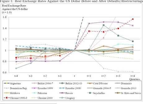
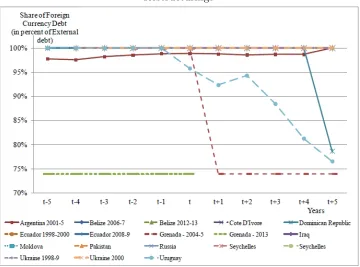
Figure 1 displays ‡uctuations of real exchange rates against the US dollar in quarterly frequency before and after defaults/announcements of restructurings from 18 episodes in 1998-2013.6 Following
de…nitions of preemptive and post-default restructurings in Asonuma and Trebesch (2013), we settat time of defaults for post-default restructuring cases and at time of announcements of restructurings for preemptive episodes.78 Real exchange rates are normalized with respect to levels at the time of
2Burger and Warnock (2006) stress that by improving policy performance and strengthening institutions, emerging
economies may develop the local currency bond market, reduce their currency mismatch and lessen the likelihood of future crises.
3Aghion, Bacchetta, and Banerjee (2004) propose the following: borrowers can use unsecured debt in domestic
currency as collateral to obtain a loan in foreign currency. This reduces the interest rate on foreign currency debt since, in the case of a crisis, the loss is partially transferred to lenders in domestic currency.
4In addition, Corsetti and Mackowiak (2004) show how monetary and …scal policies, including maturity and currency
denomination of debt, interact to determine the dynamic response of the economy and magnitude of devaluation and in‡ation.
5We relate our paper to the literature on portfolio allocation between an emerging market economy and an advanced
economy as in Devereux and Sutherland (2009) and Tille and Van Wincoop (2010), which examine determinants of optimal risk-sharing allocations. Coeurdacier and Gourinchas (2013) consider international portfolio with real exchange rate and non-…nancial risks that account for observed levels of equity home bias.
6We exclude episodes of default/debt restructurings of external debt held by o¢cial creditors because of the absence
of precise data on defaults and announcements of restructurings. Moreover, for default/restructuring of external debt held by private creditors, cases of Antigua and Barduba, Serbia and Montenegro, and Iraq are not included due to a lack of quarterly data on both nominal exchange rates and CPI. The case of Greece is not included in our sample due to the absence of nominal exchange rate against the euro associated with Eurozone membership.
7Asonuma and Trebesch (2013) introduce a new typology of two types of sovereign debt restructurings: those
implemented prior to a unilateral payment default, which they term “preemptive,” and those where the government defaults …rst and then starts to renegotiate its debt later on, which are termed as “post-default” cases.
8An alternative approach is to use selective default (SD) ratings on foreign currency debt by Standard and Poor’s.
defaults or announcements of restructurings. We observe an empirical link between the real exchange rate depreciation and default risk (default choice): on one hand, the real exchange rate depreciation increases a burden of payments for a sovereign country and triggers a default; on the other hand, the country’s announcement of default or restructuring leads to further real exchange rate depreciation. Exceptions are Ecuador in 2008 for the pre-default period and the Dominican Republic and Ukraine 2000 for the post-default period.91011
Figure 1: Real Exchange Rates Against the US Dollar Before and After Defaults/Restructurings
9The Ecuador 2008 episode can be treated as exceptional since it announced in December 2008 that the government
missed an interest payment of $30.6 million on its $510 million of 12% global bonds due in 2012. Prior to the announce-ment, the authorities made statements in November 2008 that the 2012 and the 2030 securities were “illegal” and “illegitimate.” Therefore, default was considered to be triggered by political decision rather than solvency or liquidity concerns.
1 0The Dominican Republic in 2004-5 is also considered an outlier since it announced its debt restructuring on private
debt in April 2004, following restructuring on o¢cial sector debt. However, its debt restructuring had proceeded in two separate approaches. For bank loans, though the sovereign started its negotiation with creditors in August 2004, it missed its payments in February 2005 and launched the …nal exchange o¤er in June 2005, which was completed later in October 2005. On the contrary, for external bonds, after negotiation was initiated in January 2005, the sovereign launched the …nal exchange o¤er in April 2005 and completed the exchange later in May 2005.
1 1In the case of Ukraine 2000, the real exchange rate had been on a depreciation trend for 9 quarters until its peak in
Source: Asonuma and Trebesch (2013), IMF IFS
2.2 Empirical Analysis of the Link
With our sample of 18 episodes, empirical analysis attempts to examine a relationship between real exchange rate depreciations and default probability (default choice) in both pre-default and post-default periods.12 First, in pre-default periods, we explore whether the level of lagged real exchange rates leads to an increase in default probability. Our sample is in quarterly frequency, and each episode covers periods from 5 quarters before to time of defaults/announcement of restructurings. For a proxy for default probability, we use credit ratings on foreign currency debt, which are transformed into discrete forms following Sy (2002).1314 One advantage of this approach is to capture the high
degree of variation in default probability. Since lagged real exchange rates are normalized, with respect to their level at defaults/announcement of restructurings, these series re‡ect the magnitude of depreciations towards the levels at default/announcement of restructurings.15 Given the possibility of an endogeneity problem, we apply a two-step generalized method of moment (GMM) estimation using both US GDP deviation from the trend and the US Treasury bill rate as instruments for lagged real exchange rates. These instruments have enough explanatory power, as shown in high Adj R2
reported in Table A1 in Appendix 2. Our speci…cation is the following:
Ratingt=ERt 1 +Zt 1 +Zt 0+"1;t (1)
whereERt 1are estimates of lagged real exchange rates,Zt 1andZtare vectors of other explanatory
variables at time t 1 and t, respectively. Our choice of control variables has been guided by the literature on sovereign debt crises and is especially close to Kohlscheen (2009) and Dreher and Walter (2010). We include GDP growth rates, debt service-to-GDP, an indicator of institutional quality, and 1-year LIBOR rates in baseline speci…cation, which are found to be key factors in the sovereign debt crisis literature. An indicator of the IMF program is also added to the list since whether or not an
1 2Details and sources of variables used in empirical analysis are reported in Appendix B.
1 3The alternative approach is to use a binary variable showing default and non-default choices and to apply a probit
estimation. This method also provides results similar to Table 1, with a smaller degree of signi…cance. Our approach enables us to receive bene…ts of better …ts derived by sovereign risk ratings, which capture the high degree of variation in default probability.
1 4Sy (2002) convert S&P’s and Moody’s ratings to numerical values using a linear scale from 0 to 20 with S.D. and
CC/Ca ratings corresponding to values of 0 and 1, respectively, and AAA/Aaa ratings being assigned a value of 20.
IMF-supported program is put in place a¤ects defaults or restructurings.
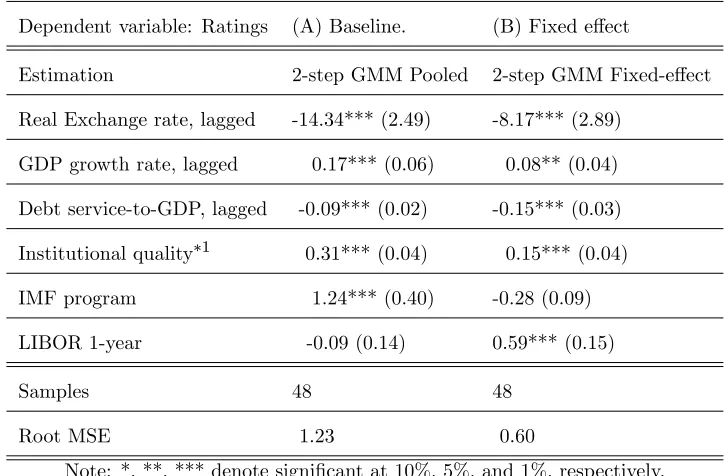
[image:9.612.123.486.335.573.2]Baseline pooled regression results (2nd column) con…rm that the real exchange rate depreciation (lagged) increases default probability: depreciations, expressed by higher levels of real exchange rates entered with lagged, lead to lower levels of ratings implying higher default probability/default choice. In line with empirical …ndings in the sovereign debt crisis literature, default probability is high if GDP growth is low and debt burden (debt service-to-GDP) is high. This is consistent with …ndings in theoretical literature of sovereign debt and defaults using one-period bonds. Moreover, when an indicator of institutional quality is low and a sovereign does not have an IMF-supported program, the sovereign is more likely to default. The results are robust if we attempt to re‡ect heterogeneity in sovereign risk ratings by applying …xed e¤ect regression (3rd column). All relevant variables, except an indicator of the IMF program, remain in expected signs with signi…cance.
Table 1: Regression Results for the Pre-Default Period
Dependent variable: Ratings (A) Baseline. (B) Fixed e¤ect
Estimation 2-step GMM Pooled 2-step GMM Fixed-e¤ect
Real Exchange rate, lagged -14.34*** (2.49) -8.17*** (2.89)
GDP growth rate, lagged 0.17*** (0.06) 0.08** (0.04)
Debt service-to-GDP, lagged -0.09*** (0.02) -0.15*** (0.03)
Institutional quality 1 0.31*** (0.04) 0.15*** (0.04)
IMF program 1.24*** (0.40) -0.28 (0.09)
LIBOR 1-year -0.09 (0.14) 0.59*** (0.15)
Samples 48 48
Root MSE 1.23 0.60
Note: *, **, *** denote signi…cant at 10%, 5%, and 1%, respectively.
1Institutional quality is the quarterly average of monthly PRC composite risk ratings from 1985-2012, with
100 and 0 as the highest and lowest indices, respectively.
Ratings on sovereign bonds are treated as indicators of default choices.16 The same method of a two-step GMM regression is taken using credit ratings of other emerging countries in other regions with a similar size and degree of openness and quality of institution as instruments for lagged default probability. High Adj R2 in Table A2 in Appendix B con…rms high explanatory power of these
instruments. We apply the following speci…cation:
ERt=Ratingt 1 +Zt +Zt 1 0+"2;t (2)
where Ratingt 1 are estimates of lagged ratings, Zt 1 and Zt are vectors of other explanatory
vari-ables at time t 1 and t, respectively. For choice of control variables, we follow the literature on determinants of real exchange rates, especially Maeso-Fernandez et al. (2001) and IMF (2006). The set of explanatory variables in baseline speci…cation includes GDP growth rate di¤erential, real in-terest rate di¤erential, net foreign assets-to-GDP and real oil price shock, which are considered to be dominant determinants of real exchange rates in the literature. In addition to these variables, we also include an indicator of an IMF program and 1-year LIBOR rates because real exchange rates are also in‡uenced by the conditionality under an IMF program and global liquidity.
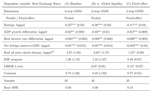
From baseline pooled regression results, we see that sovereigns’ default choices, expressed as lower credit ratings, induce real exchange rate depreciations: defaults denoted by lower levels of ratings, entered with lagged, lead to real exchange rate depreciation shown by a higher level of subsequent real exchange rates. Similar to what the literature on determinants of real exchange rates has explained, real exchange rates depreciate when GDP growth rates and real interest rates are lower than those of partner countries and the sovereign reduces net foreign assets. An increase in real oil prices, considered as terms of trade shock, leads to depreciation in real exchange rates since deterioration of the terms of trade of a country should result in a real exchange rate depreciation of that country. On the contrary, neither the IMF program nor LIBOR rates have signi…cant in‡uence over real exchange rates. Obtained results are robust, even if we apply the pooled regression with global liquidity proxied by LIBOR rates and …xed e¤ect regression.
1 6Using a binary variable showing default and non-default choices as one of the explanatory variables is an alternative
Table 2: Regression results for the Post-Default Period
Dependent variable: Real Exchange Rates (A) Baseline. (B) w. Global liquidity (C) Fixed e¤ect
Estimation 2-step GMM 2-step GMM 2-step GMM
Pooled / Fixed-e¤ect Pooled Pooled Fixed-e¤ect
Ratings, lagged -0.25*** (0.03) -0.26*** (0.03) -0.11*** (0.04)
GDP growth di¤erential, lagged -0.02** (0.009) -0.02** (0.01) -0.017** (0.009)
Real interest rate di¤erential, lagged -0.004*** (0.002) -0.004** (0.002) -0.009** (0.002)
Net foreign assets-to-GDP, lagged -0.05*** (0.013) -0.05*** (0.014) -0.053*** (0.02) Real oil price shock dummy, lagged 1 2.67 (1.62) 3.04* (1.57) 1.55* (0.90)
IMF program 1.36 (1.10) 1.53 (1.07) 0.49 (0.67)
LIBOR 1-year - 0.07 (0.05) 0.13* (0.07)
Constant 0.72 (1.06) 0.43 (1.02) 0.77 (0.55)
Samples 32 32 32
Root MSE 0.30 0.30 0.18
Note: *, **, *** denote signi…cant at 10%, 5%, and 1%, respectively.
1Real oil price shock is an indicator showing the world oil price index de‡ated by the US Producer Price
Index (PPI) for countries heavily dependent on oil prices, while 0 is given for those less dependent on oil
prices.
3
Model Environment
3.1 General Points
The basic structure of the model is in line with previous work, extending the sovereign debt model of Eaton and Gersovitz (1981).17 Our model embeds real exchange rate dynamics and currency
denomination in a two-country framework. We consider a risk-averse sovereign and a representative risk-averse creditor. Their preferences are shown by following utility functions:
E0
1
X
t=0 tu(c
t); E0
1
X
t=0
( )tu(ct)
1 7Our incomplete market assumption of capital market under the two-country framework follows Benigno and
where 0 < < 1 is a discount factor of the sovereign, and 0 < < 1 is a discount factor of the creditor. ct and ct denote consumptions of borrower and lender in period t, and u(:) is one-period
utility function, which is continuous, strictly increasing and strictly concave, and satis…es the Inada conditions. A discount factor of the sovereign re‡ects both pure time preference and probability that the current sovereignty will survive into next period, whereas a discount factor of the creditor shows only pure time preference. An assumption of a risk-averse creditor is in line with the behavior of investors in emerging …nancial markets, who prefer to avoid real exchange rate risks.18
All information on income processes of two parties and bond issuances is perfect and symmetric. In each period, the sovereign starts with total debt bt, a fraction dominated in local currency bt,
and the remaining denominated in foreign currency (1 )bt. We provide a brief explanation of …xed
share of foreign currency debt in Section 3.3.
Both the sovereign and creditor receive stochastic endowment streams of tradable goods yT t,
yT
t and non-tradable goods yNt , ytN . We denote yt, a column vector of four income processes:
yt= yTt; ytT ; ytN; ytN . It is stochastic, drawn from a compact setY = yminT ; yTmax yminT ; ymaxT
yN
min; ymaxN yminN ; ymaxN R4+. (yt+1jyt) is probability distribution of a vector of shocks yt+1
conditional on previous realization yt. Both sovereign and creditor consume not only non-tradable
goods, but also two types of tradable goods endowed in each country. They export their own endowed tradable goods and import tradable goods endowed in the counterpart’s country. When the sovereign repays its debt and issues new debt, it can import tradable goods endowed in the creditor’s country more than its exports of tradable goods, i.e. having the current account de…cit. On the contrary, when the sovereign defaults, it only imports tradable goods endowed in the creditor’s country equal to its exports of tradable goods, i.e. having the current account balanced.
The representative creditor is risk-averse. As mentioned above, it is also subject to stochastic income shocks and opts to smooth its consumption through lending/borrowing to the sovereign. The risk-averse creditor prefers to avoid real exchange rate risks and opts to issue bonds in their local
1 8Lizarazo (2013) explains that assumption of risk-averse creditors seems to be justi…ed by characteristics of the
currency. A large fraction of external debt denominated in foreign currency, shown in Section 3.3, also re‡ects behavior of a risk-averse creditor. Risk-averseness, rather than risk-neutrality, is necessary for determination of real exchange rate depending not only on the sovereign’s but also the creditor’s income shocks.
The international capital market is incomplete. The sovereign and creditor can borrow and lend only via one-period, zero-coupon bonds indexed to their consumer price index (CPI), and there are two types of bonds the sovereign (creditor) issues: bonds denominated in local and foreign currency. bt+1
(bt+1) denotes the amount of bonds to be repaid next period whose set is shown byB = [bmin; bmax]
Rwherebmin 0 bmax. We set the lower bound atbmin < yTmax=r , which is the largest debt that
the sovereign could repay. The upper bound bmax is the high level of assets that the sovereign may
accumulate.19 The upper bound is the highest level of assets that the sovereign can accumulate, and the lower bound is the highest level of debt that it can hold. We assume qi(b
t+1; yt) (i2 fH; Fg) to
be the price of bonds with asset position bt+1 and a vector of income shocksyt. We assume thatqH
and qF are denominated in local and foreign currency, respectively. Price functions of both bonds
are determined in equilibrium.
We de…ne the current real exchange rate et as units of local currency against one unit of foreign
currency as in Walsh (2003). An increase in et means one unit of domestic currency buys fewer units
of foreign currency. Thus, a rise in et corresponds to a fall in the value of domestic currency, i.e.
depreciation of domestic currency. The real exchange rate is also determined in equilibrium together with bond prices.
We assume that the creditor always commits to repay its debt. However, the sovereign is free to decide whether to repay its debt or to default. If the sovereign chooses to repay its debt, it will preserve its status to issue bonds next period. On the contrary, if it chooses not to pay its debt, it is then subject to both exclusion from the international capital market and direct output costs. The sovereign su¤ers symmetric output costs on tradable and non-tradable goods. This assumption is consistent with none of the empirical …ndings justifying asymmetric output costs across tradable and non-tradable sectors in the literature of costs of sovereign defaults.20 We consider that the debtor
1 9b
max exists when the interest rates on the sovereign’s savings are su¢ciently low compared to the discount factor,
which is satis…ed as(1 +r ) <1:
2 0Though it is within the manufacturing goods sector, not across the tradable and non-tradable goods sectors,
defaults total external debt (bt). Defaulting total external debt is supported by evidence on recent
external debt restructurings, where sovereigns default on both local and foreign currency debt issued at the international market.21
When a default is chosen, the sovereign will be in temporary autarky. After being excluded from the market for one period, with exogenous probability , it will regain access to the market. Otherwise, it will remain in …nancial autarky next period.
3.2 Timing of the Model
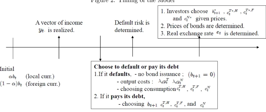
[image:14.612.73.539.284.480.2]Timing of decisions within each period is summarized in Figure 2.
Figure 2: Timing of the Model
The sovereign starts the current period with total debtbt, comprised of local and foreign currency
debt. After observing a vector of income shocks yt, the sovereign chooses either to pay its debt or to
default.
If the sovereign chooses to pay the total debt, given bond price schedules and the real exchange rate, it chooses next period total debtbt+1 and current consumptioncT;Ht ,c
T;F
t andcNt . Then, default
probability is determined. Given bond prices and the real exchange rate, the creditor chooses bt+1
consistent with the belief of default probability, and consumption cT ;Ht ,cT ;Ft ;and cN
t . Bond prices
together with the real exchange rate are determined in equilibrium.
2 1There are only a few episodes where sovereigns apparently di¤erentiate creditors of foreign currency and local
On the contrary, if the sovereign opts to default, it su¤ers direct output costs due to default dytT
and dyNt . The debtor will be in …nancial autarky and cannot raise funds at the international capital
market this period (bt+1 = 0). It simply chooses its current consumption cT;Ht , c T;F
t and cNt . Only
the real exchange rate (et) is determined at equilibrium.
3.3 Fixed Share of Foreign Currency Debt
We explain, succinctly, a rationale of assumption on share of foreign currency debt. Figure 3 shows shares of foreign currency debt in annual frequency before and after defaults and restructurings for 18 episodes from 1999-2013.22 We compute shares of foreign currency debt for 18 episodes using data
of international bond issuance from Bloomberg and Dealogic.23 A majority of countries, which have
experienced defaults or restructurings recently, had a large fraction of their external debt, close to 100 percent, denominated in foreign currency both before and after defaults and restructurings. Even among four exceptional cases, three episodes, such as the Dominican Republic in 2004-5, Grenada in 2004-5 and Uruguay in 2003, witnessed a decrease in share of foreign currency denominated debt only after defaults or announcements of restructurings. In addition, these countries seldom changed shares of foreign currency debt, as shown in limited variations over the sample period in Figure 3.24
These clearly support our assumption of …xed and high shares of foreign currency debt.
2 2Data on bond issuances for Dominica and St. Kitts and Nevis are not available.
2 3Due to a lack of currency denomination data on loans from Dealogic, our computed shares are based only on bond
issuances.
2 4Small variance in share of foreign currency denominated debt over the sample period reported in Table A1 in
Figure 3: Share of Foreign Currency Debt Before and After Defaults or Announcements of Restructurings
Source: Asonuma and Trebesch (2013), Bloomberg and Dealogic.
4
Recursive Equilibrium
In this section, we de…ne the stationary recursive equilibrium of the model. Our framework incor-porates three key features: (1) optimal behavior of a risk-averse foreign creditor, (2) two types of external bonds denominated in local and foreign currencies, and (3) endogenous determination of real exchange rate in equilibrium.
4.1 The Sovereign Country’s Problem
The country’s problem is to maximize the expected lifetime utility given by
E0
1
X
t=0 tu(c
t) (3)
A consumption basketct is de…ned by the CES aggregates of consumption shown as
ct= h
where cT
t and cNt are consumptions of tradable and non-tradable goods, and is the elasticity of
intratemporal substitutions between these goods. The tradable component is, in turn, comprised of local and foreign-endowed goods in the following manner:
cTt =h 1(cT;Ht ) 1 + (1 )1(cT;Ft ) 1i 1 (5)
where cT;Ht and cT;Ft are consumptions of traded goods endowed in the country and the creditor’s country, respectively. is the elasticity of intratemporal substitution between traded goods endowed in the country and the creditor’s country.
Corresponding to the CES bundles of consumption goods, we have an isomorphic price index:
pt= !(pTt)1 + (1 !)(pNt )1 1 1
(6)
where pT
t and pNt are prices of traded and non-traded goods. The price of tradable goods is the
numeraire (pT
t = 1). The tradable good price is, in turn, comprised of prices of local and
foreign-endowed goods:
1 =h (pT;Ht )1 + (1 )(etpT;Ft )1 i 1
1
(7)
where pT;Ht andpT;Ft are prices of traded goods endowed in each country.
Let V(bt; yt) be the lifetime value function of the country that starts the current period with
initial assets bt and a vector of income shocks yt. Given sovereign bond prices qi(bt+1; yt) i= H; F
and the real exchange rate et, the country solves its optimization problem.
If the country decides to pay its debt, it chooses its next-period assets (bt+1) and current
con-sumption after paying back its initial debt. On the contrary, if the country defaults, it will not be able to issue bonds in the current period. It simply chooses current consumption.
Given its option to default, V(bt; yt) satis…es
where VR(b
t; yt) is its value, which the country chooses to pay debt given as
VR(bt; yt) = max cT ;Ht ;c
T ;F t ;cNt ;bt+1
u(ct) + Z
Y
V(bt+1; yt+1)d (yt+1jyt) (9)
s:t: pT;Ht cT;Ht +etpT;Ft c T;F
t +pNt cNt +pt qH(bt+1; yt) +etqF(bt+1; yt)(1 ) bt+1
= pT;Ht yTt +pNt yNt +pt[ +et(1 )]bt
s:t: (4) & (5)
and VD(y
t) is the value, which the country decides to default, shown as
VD(yt) = max cT ;Ht ;cT ;Ft ;cN
t
u(ct) + 2
4 Z
Y
V(0; yt+1)d (yt+1jyt) + (1 ) Z
Y
VD(yt+1)d (yt+1jyt) 3
5 (10)
s:t: pT;Ht cT;Ht +etpT;Ft c T;F
t +pNt cNt = (1 d)ptT;HytT + (1 d)pNt yNt
s:t: (4) & (5)
where V(0; yt+1) is its value next period with no initial debt. dpT;Ht yTt and dpNt ytN express output
costs, which the country su¤ers due to a default. When the country decides the next-period assets, it also takes into consideration impacts of the real exchange rate, which is determined by optimality conditions of the sovereign debtor and the creditor.
The country’s default policy can be characterized by default set D(bt) Y. The default set is a
set of income vectors y’s for which default is optimal given the debt position bt.
D(bt) = yt2Y :VR(bt; yt)< VD(yt) (11)
cT;Ht cT;Ft = 1
pT;Ht etpT;Ft
!
(13)
qH(bt+1; yt) +etqF(bt+1; yt)(1 ) =Et
u0(c
t+1)
u0(c
t)
1N on Def ault[ +et+1(1 )] (14)
On the contrary, if the country chooses to default, we have equation (12) and (13), not (14).
4.2 The Foreign Creditor’s Problem
The foreign creditor is also risk-averse and behaves competitively at the market. The problem is maximizing its expected lifetime utility given by
E0
1
X
t=0
( )tu(ct) (15)
Its consumption basketct is similar to that of the country:
ct =h(! )1 (cTt ) 1 + (1 ! )1(cNt ) 1i 1 (16)
where cT
t and cNt are consumptions of traded and non-traded goods. Tradable goods consumption
is composed of consumptions of two tradable goods: cT ;Ht and cT ;Ft :
cTt =h( )1 (cT ;Ht ) 1 + (1 )1(cT ;Ft ) 1i 1 (17)
Corresponding to the CES bundles of consumption goods, we have an isomorphic price index:
pt =h(! ) (pTt )1 + (1 ! )(pNt )1 i
1 1
(18)
where pT
t and pNt are prices of traded and non-traded goods. The tradable goods price of the
creditor is similar to that of the country shown as:
pTt =
2
4(1 ) p
T;H t
et !1
+ (pT;Ft )1
3
5 1 1
(19)
consumption cT ;Ht ,cT ;Ft , and cN
t subject to its budget constraint, such as
pT;Ht et
cT ;Ht +pT;Ft cT ;Ft +pNt cNt +pt 2
6 4
qH(bt +1;yt) et
+qF(b
t+1; yt)(1 ) 3
7
5bt+1 =p T ;F
t yTt +pNt ytN +pt
1
et
+ (1 ) bt
(20) Then, we obtain the following optimality conditions:
cT t cN t = ! 1 ! pT t pN t (21)
cT ;Ft cT ;Ht = 1
pT;Ft pT;Ht =et
!
(22)
qH(b t+1; yt)
et
+qF(b
t+1; yt)(1 ) =Et
u0(c
t+1)
u0(c
t)
1N on Def ault
1
et+1
+ (1 ) (23)
If the country defaults, the creditor maximizes its utility by choosing current consumptioncT ;Ht ,
cT ;Ft , and cN
t subject to its budget constraint:
pT;Ht et
cT ;Ht +pT;Ft cT ;Ft +pNt ctN =pT ;Ft yTt +pNt ytN (24)
Then, we have we have equation (21) and (22), not (23).
4.3 Bond Prices and Real Exchange Rate
Bond prices indexed to the sovereign’s and creditor’s CPIqi(b
t+1; yt)fori=H; F are functions of the
next-period assets and a vector of income shocks. If the country chooses to pay its debt, the creditor receives payo¤s equal to the face value of bonds, which is normalized to 1. If the country chooses to default, payo¤s are zero. We derive bond price functions for both the sovereign’s and the creditor’s Euler equations, which take into account the sovereign’s decision of paying its debt and defaulting.
qH(bt+1; yt) +etqF(bt+1; yt)(1 ) =Et
u0(c
t+1)
u0(c
t)
1N on Def ault[ +et+1(1 )] (25)
qH(b t+1; yt)
et
+qF(bt+1; yt)(1 ) =Et
u0(c
t+1)
u0(c
t)
1N on Def ault
1
et+1
The real exchange rate is de…ned as relative CPI between the sovereign and the creditors as
et=
pt
pt (27)
4.4 Market Clearing Conditions for Goods and Bonds
If the country repays its debt in the current period, market clearing conditions for tradable goods and non-tradable goods are
cT;Ht +cT ;Ht =yTt (28)
cT;Ft +cT ;Ft =yT
t (29)
cNt =ytN (30)
cNt =ytN (31)
On the contrary, in the case of default, the following are market clearing conditions for tradable goods and non-tradable goods endowed in the country.
cT;Ht +cT ;Ht = (1 d)ytT (28’)
cNt = (1 d)ytN (30’)
Market clearing condition for bonds is
bt+ (1 )bt = 0 (32)
where denotes the size of the sovereign economy relative to the creditor.
4.5 Recursive Equilibrium
We de…ne a stationary equilibrium in the model.
De…nition 1 A recursive equilibrium is a set of functions for (A) the country’s value func-tion V(bt; yt); consumption, cT;Ht (bt; yt), cT;Ft (bt; yt), cNt (bt; yt); asset position bt+1(bt; yt) and default
bt+1(bt; yt); and (C) bond prices qi(bt+1; yt) for i=H; F and the real exchange rate et(bt+1; yt) such
that
[1] Given bond prices and the real exchange rate, the country’s value functionV(bt; yt);
consump-tion, cT;Ht (bt; yt), cT;Ft (bt; yt), ctN(bt; yt); asset position bt+1(bt; yt); and default set D(bt) satisfy the
country’s optimization problem.
[2] Given bond prices and the real exchange rate, the creditor’s consumptioncT ;Ht (bt; yt),cT ;Ft (bt; yt),
cN
t (bt; yt) and asset positionbt+1(bt; yt) satisfy the creditor’s optimization problem.
[3] Bond bond prices qi(b
t+1; yt) for i=H; F and the real exchange rate et(bt+1; yt) satisfy
opti-mality conditions of two parties.
[4] Market clearing conditions for goods and bonds are satis…ed.
In equilibrium, default probabilityp(bt+1; yt) is related to the sovereign’s default decision in the
following manner:
p(bt+1; yt) = Z
D (bt+1)
d (yt+1jyt) (33)
Risk-free interest rate is de…ned as
1 1 +r (bt+1; yt)
= Et
u0(c
t+1)
u0(c
t)
(34)
We de…ne total spreads for domestic and foreign currency debt evaluated by the creditor’s side as follows:
sH(bt+1; yt) =
et
qH(b t+1; yt)
1 r (bt+1; yt) (35)
sF(bt+1; yt) =
1
qF(b t+1; yt)
1 r (bt+1; yt) (36)
5
Quantitative Analysis
regularities, including moments of the real exchange rates in both pre-default and post-default periods. Lastly, most importantly, the model generates the link between real exchange rate dynamics and default choices (default probability) around default.
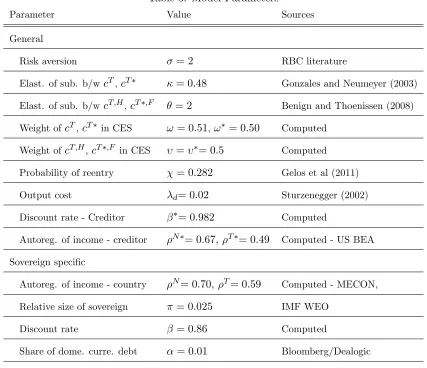
5.1 Parameters and Functional Forms,
We use most of the parameters and functional forms speci…ed in previous work. There are three new elements in the model associated with a two-country, four-goods set-up: (i) relative size of the sovereign, (ii) weights on consumption of home-endowed tradable goods, and (iii) share of domestic currency debt.
The following utility functions are used in numerical simulation:
u(ct) =
c1t
1 ; u(ct) =
ct1
1 (37)
where expresses degree of risk aversion. We set equal to 2, which is commonly used in real business cycle analysis for advanced economy and emerging markets. The creditor’s discount factor is set to = 0:982 to replicate the risk-free interest rate of 1.7%.25 The elasticity of substitution between tradable and non-tradable consumption is taken from Gonzales and Neumeyer (2003) where they estimate the elasticity for Argentina to be equal to 0.48. We assume an elasticity of substitution between tradable goods endowed in the sovereign and the creditor country , of 2, as in Benigno and Thoenissen (2008). Weights of tradable goods consumption and home-endowed tradable goods consumptions are set to ! = 0:51,! = 0:5 and = = 0:5 in order to have the price of tradable goods at steady-state distribution (pT = 1).
The probability of re-entry to credit markets after defaults is set at = 0:282, which is consistent with observed evidence regarding the exclusion from credit markets of defaulting countries mentioned in Gelos et al (2011). Output loss parameter d is assumed to be 2% following Sturzenegger (2002)’s
estimates.
We assume each exogenous endowment stream yi
t for i = fT; N; T ; N g follows a log-normal
2 5Similarly, Lizarazo (2013) set the creditor’s discount rate as = 0:98to generate the international interest rate of
AR(1) process where innovations to the shocks are allowed to be correlated:
log(yit) = log(yi) + iy log(yit 1) log(yi) + iy (38)
where yi is the mean income,E[ i
y] = 0fori=fT; N; T ; N gand the variance-covariance matrix of
the error terms is the following:
E[ 0 ] =
2 6 6 6 6 6 6 6 4
T T N T T T N
T N N N T N N
T T N T T T N
T N N N T N N
3 7 7 7 7 7 7 7 5 = 2 6 6 6 6 6 6 6 4
0:0027 0:0019 0 0
0:0019 0:0019 0 0
0 0 0:0006 0:0002
0 0 0:0002 0:0002
3 7 7 7 7 7 7 7 5 (39)
where = [ Ty; Ny ; Ty ; Ny ]0. Auto-correlation coe¢cients and the variance-covariance matrix are
computed from the quarterly real GDP data of Argentina from 1993Q1 to 2011Q4 (sovereign) and of the US from 1988Q1 to 2011Q4. Sector-level GDP data are seasonally adjusted and are taken from the Ministry of Economy and Production (MECON) and the US Bureau of Economic Analysis (BEA). The sectoral classi…cation into tradable and non-tradable goods follows the traditional approach adopted in real business cycle literature. The tradable goods sector comprises "manufacturing" and the primary sectors, whereas the non-tradable goods sector is composed of remaining sectors. The data are detrended using Hodrick-Prescott …lter with a smoothing parameter of 1600. Each shock is then discretized into a …nite state Markov chain by using a quadrature procedure in Hussey and Tauchen (1991) from their joint distribution. We obtain estimated coe¢cients such as T = 0:59and
N = 0:70for Argentina and T = 0:49 and N = 0:67 for the US.
Table 3: Model Parameters
Parameter Value Sources
General
Risk aversion = 2 RBC literature
Elast. of sub. b/wcT,cT = 0:48 Gonzales and Neumeyer (2003)
Elast. of sub. b/wcT;H,cT ;F = 2 Benign and Thoenissen (2008)
Weight ofcT,cT in CES != 0:51,! = 0:50 Computed
Weight ofcT;H,cT ;F in CES = = 0:5 Computed
Probability of reentry = 0:282 Gelos et al (2011)
Output cost d= 0:02 Sturzenegger (2002)
Discount rate - Creditor = 0:982 Computed
Autoreg. of income - creditor N = 0:67, T = 0:49 Computed - US BEA Sovereign speci…c
Autoreg. of income - country N= 0:70, T= 0:59 Computed - MECON, Relative size of sovereign = 0:025 IMF WEO
Discount rate = 0:86 Computed
Share of dome. curre. debt = 0:01 Bloomberg/Dealogic
5.2 Numerical Results on Equilibrium Properties
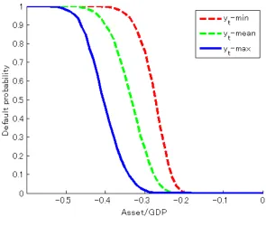
Figure 4: Default Probability
Figure 5: Real Exchange Rates
[image:26.612.151.446.93.344.2]to lower consumption of tradable goods (with less tradable goods endowment left for consumption) indicating higher marginal utility of consumption. This, in turn, results in both the lower price of tradable goods and the lower overall price. On the contrary, when the sovereign defaults at current debt, the real exchange rate tends to depreciate. By defaulting, the sovereign prefers to have higher consumption of tradable goods, indicating lower marginal utility of consumption, which leads to both a higher price of non-traded goods and a higher overall price level.
Moreover, the level of the real exchange rate is high implying depreciation when the sovereign has a low level of traded goods. With a low level of traded goods, the sovereign tends to accumulate higher debt which leads to an increase in default probability. Then, the real exchange rate depreciates and is associated with an increase in default probability. Price functions for newly-issued debt and debt level are shown in Appendix C.
5.3 Simulation - Argentina
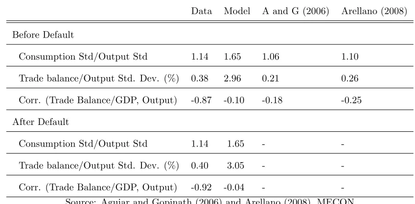
We conduct 1000 rounds of simulations, with 2000 periods per round and then extract the last 200 periods to analyze features evaluated at the steady-state distribution. In the last 200 periods, we choose 40 observations before and after a default event to compare with moments in data for Argentina. The second column in Table 4 and 5 summarizes moments of data.26 Output data are
seasonally adjusted from the MECON for 1993Q1-2001Q3 and 2001Q4-2011Q4. Trade balance is calculated as ratio to GDP. Argentina’s external debt data are from the IMF WEO for 1993-2001 and 2002-2011. We calculate two measures of the sovereign’s indebtedness; the …rst measure is the average external debt to GDP ratio. We also compute the ratio of the country’s debt service (including short-term debt) to its GDP for Argentina. Bond spreads are from the J.P. Morgan’s Emerging Market Bond Index (EMBI) Global for Argentina for 1998Q1-2001Q3 and 2001Q4-2011Q4. Real exchange rate is computed based on monthly Argentina nominal exchange rates against the US dollar, Argentina CPI, and US CPI from IMF IFS for 1993Q1-2001Q3 and 2001Q4-2011Q4. We compare our simulation results with those of Aguiar and Gopinath (2006) and Arellano (2008).
As is obvious in Table 5, the model matches business cycle statistics in data in both pre-default and post-default periods. Our model replicates volatile consumption and trade balance/GDP volatility, both of which are prominent features of emerging economy business cycle models as in Aguilar and
Gopinath (2007) and Neumeyer and Perri (2005). Trade balance/output standard deviation in the model is much higher than that of data because trade balance in our model also includes variations of imports merely driven by real exchange rate ‡uctuations. Moreover, it also generates a negative correlation between trade balance and output.
Table 4: Business Cycle Statistics for Argentina
Data Model A and G (2006) Arellano (2008)
Before Default
Consumption Std/Output Std 1.14 1.65 1.06 1.10
Trade balance/Output Std. Dev. (%) 0.38 2.96 0.21 0.26
Corr. (Trade Balance/GDP, Output) -0.87 -0.10 -0.18 -0.25
After Default
Consumption Std/Output Std 1.14 1.65 -
-Trade balance/Output Std. Dev. (%) 0.40 3.05 -
-Corr. (Trade Balance/GDP, Output) -0.92 -0.04 - -Source: Aguiar and Gopinath (2006) and Arellano (2008), MECON
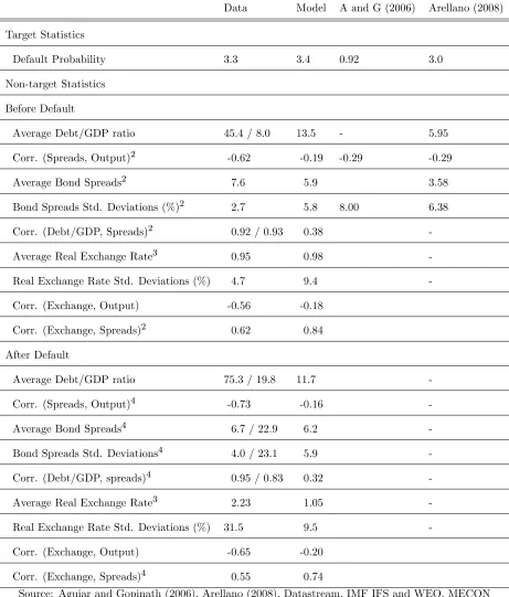
On non-business cycle statistics, the model shows relations among bond spreads, debt/GDP ratio and output, as in the data in both pre-default and post-default periods. Bond spreads are positively correlated with debt/GDP ratio, but negatively correlated with output. This is because default probability is high, leading to higher spreads when debt/GDP ratio is high and output is low. Our simulation also reproduces similar levels of average bonds spreads and volatility of spreads in both pre-default and post-default periods, though simulated moments in post-default periods are closer to those in the data. However, we see some deviations of average debt/GDP ratio from the total debt service/GDP ratio in data in both pre-default and post-default periods.
pre-default period, whereas it is 9.4%, much lower than data (27.6%) in the post-default period.
Table 5: Non-Business Cycle Statistics for Argentina (in quarterly frequency)1
Data Model A and G (2006) Arellano (2008)
Target Statistics
Default Probability 3.3 3.4 0.92 3.0
Non-target Statistics
Before Default
Average Debt/GDP ratio 45.4 / 8.0 13.5 - 5.95
Corr. (Spreads, Output)2 -0.62 -0.19 -0.29 -0.29
Average Bond Spreads2 7.6 5.9 3.58
Bond Spreads Std. Deviations (%)2 2.7 5.8 8.00 6.38
Corr. (Debt/GDP, Spreads)2 0.92 / 0.93 0.38
-Average Real Exchange Rate3 0.95 0.98
-Real Exchange Rate Std. Deviations (%) 4.7 9.4
-Corr. (Exchange, Output) -0.56 -0.18
Corr. (Exchange, Spreads)2 0.62 0.84
After Default
Average Debt/GDP ratio 75.3 / 19.8 11.7
-Corr. (Spreads, Output)4 -0.73 -0.16
-Average Bond Spreads4 6.7 / 22.9 6.2
-Bond Spreads Std. Deviations4 4.0 / 23.1 5.9
-Corr. (Debt/GDP, spreads)4 0.95 / 0.83 0.32
-Average Real Exchange Rate3 2.23 1.05
-Real Exchange Rate Std. Deviations (%) 31.5 9.5
-Corr. (Exchange, Output) -0.65 -0.20
Corr. (Exchange, Spreads)4 0.55 0.74
Source: Aguiar and Gopinath (2006), Arellano (2008), Datastream, IMF IFS and WEO, MECON
1 Spreads corresponds to spreads on foreign currency denominated bonds.
3 Over 10 quarters
4 Excluding autarky periods.
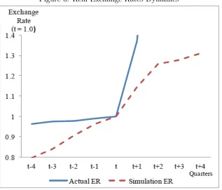
[image:30.612.150.467.406.677.2]Figure 6 contrasts the simulated process with the actual dynamics of the real exchange rate of Argentina before and after default. We replicate two features of real exchange rate movements around defaults. In the model, before defaults, the sovereign receiving a series of low traded goods shocks, tends to accumulate more debt and faces real exchange rate depreciation. Since a majority of debt is denominated in foreign currency, this, in turn, increases the burden of payments in terms of local currency, increasing default probability and forcing the sovereign to default. Once the sovereign de-clares default, it su¤ers output costs due to default and loses access to the market. By defaulting, the sovereign enjoys higher consumption of traded goods, indicating a lower marginal utility of consump-tion, which leads to both a higher price of non-traded goods and a higher overall price level. Thus, it results in a further depreciation of the real exchange rate. This mechanism drives the equilibrium depreciation of real exchange rate in the model and it is a plausible explanation of observed pattern in the data.
Figure 6: Real Exchange Rates Dynamics
We compare simulated moments of spreads on domestic and foreign currency bonds in the post-default periods with data.27 The current model replicates a common feature that average spreads on domestic currency bonds are higher than those of foreign currency bonds, incorporating real exchange rate ‡uctuations as we see in the data. Average bond spreads for domestic currency bonds in our model are three times as high as those of foreign currency bonds. In addition, we also generate much more volatile domestic currency bonds than foreign currency bonds as observed in the data. Both real exchange rate ‡uctuations and investor risk aversion interact and produce high and volatile domestic currency bond spreads.
Table 6: Statistics for Bond Spreads in Post-default Periods
After Default Data1 Model
Domestic currency debt
Average Bond Spreads 26.4 20.3 Bond Spreads Std. Dev.(%) 15.7 10.5 Foreign currency debt
Average Bond Spreads 6.7 / 22.9 6.2 Bond Spreads Std. Dev.(%) 4.0 / 23.1 5.9
Sources: Author’s calculations and Bloomberg
1 For domestic currency debt, data are from 2009M1 to 2011M5.
5.4 Comparison with the Model of a Risk-neutral Creditor
To understand the role of a creditor’s risk aversion, we contrast moments of bond spreads to those under a conventional sovereign debt model with a risk-neutral creditor, as in Aguiar and Gopinath (2006) and Arellano (2008). As reported in Table 8, average bond spreads in the current model are higher and closer to the data than those in a model with a risk-neutral creditor in both pre- and post-default periods. Moreover, the current model generates higher standard deviations of bond spreads than the model with a risk-neutral creditor. These are associated with high average bond spreads, since we assume no spreads when the sovereign is in autarky.
What drives a large di¤erence in average bond spreads is the risk aversion of the creditor. Both
2 7Given the lack of spreads data on domestic currency bonds before 2009M1, we focus on moments of spreads in
average bond spreads and the standard deviation in the current model are higher and closer to the data than those in a traditional sovereign debt model with a risk-neutral creditor. In a standard model with a risk-neutral creditor, bond spreads do not include any spread premia since bond prices are simply determined by default probability. On the contrary, in the current model with the risk-averse creditor, bond prices are determined by interaction between stochastic discount factors and expected payo¤, as shown in equation (25) and (26). Risk premia, due to risk aversion of the creditor, are included in bond spreads and increase spreads close to the data.
Table 7: Statistics for Bond Spreads
Data Baseline Model - Risk-neutral creditor
Before Default
Average Bond Spreads 7.6 5.9 1.1 Bond Spreads Std. Dev.(%) 2.7 5.8 2.4 After Defaults/Restructurings
Average Bond Spreads 6.7 / 22.9 6.2 0.8 Bond Spreads Std. Dev.(%) 4.0 / 23.1 5.9 2.0
Sources: Author’s computations and Bloomberg
6
Model Implications
In this section, we explore determinants of real exchange rate dynamics. Key parameters in‡uencing real exchange rate dynamics include income processes, elasticity of substitution, and share of foreign currency debt. Hence, we …rst report the e¤ects of income processes on default probability and real exchange rate moments. We then examine in‡uence of share of foreign currency debt.
6.1 Volatility of Income Processes and Real Exchange Rate Dynamics
Table 8 reports key moment statistics under di¤erent values of the standard deviation of endowments
T and N, elasticity of substitution between tradable and non-tradable goods and discount rate
, leaving other parameters at their benchmark values.
more debt resulting in frequent defaults. Real exchange rate moments are similar to those in the baseline case.
When tradable and non-tradable goods are highly substitutable ( = 2:5), the sovereign can smooth volatility of consumption of tradable goods by substituting with non-tradable goods. This results in a smaller change in marginal substitution of consumption, leading to a smaller change in the real exchange rate. Therefore, real exchange rate depreciation and volatility are smaller than those under the benchmark case.
[image:33.612.65.588.351.608.2]Volatile income processes for both traded and non-traded goods result in higher default probability and lower level of debt. Due to an increase in volatility of income realization, the sovereign tends to default more frequently with a lower level of debt. Through positive correlation between the real exchange rate and spreads, volatile income processes for both traded and non-traded goods relate to high standard deviations of the real exchange rate in both pre-default and post-default periods.
Table 8: Model Statistics for Argentina (in quarterly frequency)
Baseline T N
0.80 0.96 0.8 2.5 0.02 0.058 0.02 0.058
Default probability (%) 3.4 3.8 1.6 1.8 0.5 1.9 3.9 2.0 4.7
Before Default
Average Debt/GDP (%) 13.5 16.6 3.0 21.2 33.2 16.7 12.7 15.0 13.0
Average Real Exchange Rate 0.98 0.98 1.02 0.98 0.99 0.98 0.98 0.98 0.97
Real Exchange Rate Std. Dev. (%) 9.4 9.3 8.8 5.8 1.9 7.6 9.9 8.1 10.3
After Default
Average Debt/GDP (%) 11.7 14.4 3.1 19.1 32.1 15.1 11.1 13.3 11.3
Average Real Exchange Rate 1.05 1.05 1.04 1.02 1.00 1.03 1.05 1.04 1.05
Real Exchange Rate Std. Dev (%) 9.5 9.5 8.6 5.9 1.9 7.6 9.8 8.1 10.3 Source: Author’s calculation
6.2 Share of Foreign Currency Bonds and Real Exchange Rate
exchange rate in post-default periods; if the sovereign issues more debt in domestic currency (1 = 0:5), one-percentage real exchange rate depreciation does not increase much burden of payments in terms of local currency, reducing default probability. The smaller share of foreign currency debt also results in higher average debt. On the contrary, standard deviations of real exchange rate are similar to those under a large share of foreign currency debt.
Table 9: Model Statistics for Argentina (in quarterly frequency) Share of foreign currency debt
1 = 0:5 1 = 0:75 1 = 0:99
Default probability (%) 3.05 3.2 3.4 Before Default
Average Debt/GDP ratio (%) 17.9 15.3 13.5 Average Real Exchange Rate 0.965 0.973 0.98 Real Exchange Rate Std. Dev. (%) 9.8 9.7 9.4 After Default
Average Debt/GDP ratio (%) 15.6 13.5 11.7 Average Real Exchange Rate 1.037 1.04 1.05 Real Exchange Rate Std. Dev (%) 9.8 9.7 9.5
Source: Author’s calculation
7
Conclusion
Emerging countries experience real exchange rate depreciations around default events. This paper attempts to explore this observed evidence within a dynamic stochastic general equilibrium model in which bond issuance in local and foreign currencies is explicitly embedded and the real exchange rate and default risk are determined endogenously. Our quantitative analysis using data of Argentina, replicates a link between real exchange rate depreciation and default probability before and after defaults.
currency, increasing default probability and forcing the sovereign to default. Once the sovereign declares default, it su¤ers output costs due to default and loses access to the market. By defaulting, the sovereign prefers to have a higher consumption of traded goods indicating lower marginal utility of consumption, which leads to both a higher price of non-traded goods and a higher overall price level. Thus, the default ends up with a further depreciation of the real exchange rate. This mechanism drives the equilibrium depreciation of real exchange rate in the model, and it is a plausible explanation of the observed pattern in the data.
So far, we have analyzed the endogenous real exchange rate dynamics before and after the default in the framework, where income processes are exogenous and output cost is …xed. It will be possible to consider interactions between real exchange rate depreciation and output costs due to default as in Mendoza and Yue (2012). This might be a potential area future research could explore.
References
[1] Aghion, P., and Bacchetta, P., and A. Banerjee, 2004, "A Corporate Balance-sheet Approach to Currency Crises," Journal of Economic Theory, Vol. 119(1), pp.6-30.
[2] Aguiar, M., and G. Gopinath, 2006, "Defaultable Debt, Interest Rates and the Current Account,"
Journal of International Economics, Vol.69(1), pp.64-83.
[3] Aguiar, M., and G. Gopinath, 2007, "Emerging Market Business Cycle: The Cycle is the Trend,"
Journal of Political Economy, Vol.115(1), pp.69-102.
[4] Arellano, C., 2008, "Default Risk and Income Fluctuations in Emerging Economies,"American Economic Review, Vol.98(3), pp.690-712.
[5] Arellano, C., and J. Heathcote, 2010, "Dollarization and Financial Integration," Journal of Economic Theory, Vol. 145(3), pp.944-973. .
[6] Asonuma, T., 2012, "Serial Default and Debt Renegotiation," forthcoming IMF Working Paper.
[8] Benigno, G., and C. Thoenissen, 2008, "Consumption and Real Exchange Rates with Incomplete Markets and Non-Traded Goods,"Journal of International Money and Finance, Vol.27, pp.926-948.
[9] Benjamin, D., and M. Wright, 2009, "Recovery Before Redemption? A Theory of Delays in Sovereign Debt Renegotiations," manuscript, University of Southhampton.
[10] Bi, R., 2008, ""Bene…cial" Delays in Debt Restructuring Negotiations," IMF working paper No.WP/08/38, International Monetary Fund.
[11] Borensztein E., and U. Panizza, 2010, "Do Sovereign Defaults Hurt Exports?" Open Economic Review, Vol.21(3), pp.393-412.
[12] Borri, N., and A. Verdelhan, 2009, "Sovereign Risk Premia," manuscript, LUISS.
[13] Burger, J., and F. Warnock, 2006, "Local Currency Bond Market," IMF Sta¤ Papers, Vol. 53, Special Issue.
[14] Bussiere, M., Fratzscher, M., and W. Koeniger, 2004, "Currency Mismatch, Uncertainty, and Debt Structure," ECB Working Paper No.0409.
[15] Chamon, M., and R. Hausmann, 2004, "Why Do Countries Borrow the Way They Borrow?" in B. Eichengreen and R. Hausmann eds., Other People’s Money - Debt Denomination and Financial Instability in Emerging Market Economies, University of Chicago Press.
[16] Chari, V.V., Kehoe, P., and E. McGrattan, 2002, "Can Sticky Price Models Generate Relative and Persistent Real Exchange Rates?" Review of Economic Studies, Vol.69, pp.633-663.
[17] Coeurdacier, N., and P.O. Gourinchas, 2013, "When Bonds Matter: Home Bias in Goods and Assets" manuscript, SciencePo.
[18] Corsetti, G., and B. Mackowiak, 2004, "A Fiscal Perspective on Currency Crises and Original Sin," in B. Eichengreen, and R. Hausmann, eds., Other People’s Money - Debt Denomination and Financial Instability in Emerging Market Economies, University of Chicago Press.
[20] Dreher, A. and S. Walter, 2010, "Does the IMF help or hurt? The E¤ect of IMF Program on the Likelihood and Outcomes of Currency Crises," World Development, Vol. 38(1), 1-18.
[21] Eaton, J. and M. Gersovitz, 1981, "Debt with Potential Repudiation: Theoretical and Empirical Analysis,"Review of Economic Studies, Vol.48, pp.289-309.
[22] Eichengreen, B., Hausmann, R., and U Panizza, 2004, "The Mystery of Original Shin" in B. Eichengreen and R. Hausmann (eds.),Debt Denomination and Financial Instability in Emerging Market Economies, Chicago, University of Chicago Press.
[23] Gelos, G., Sahay, R., and G. Sandleris, 2011, "Sovereign Borrowing in Developing Countries: What Determines Market Access?"Journal of International Economics, Vol.83(2), pp.243-254.
[24] Hussey, R., and G. Tauchen, 1991, "Quadrature-Based Methods for Obtaining Approximate Solutions to Nonlinear Asset Pricing Models,"Econometrica, Vol.59(2), pp.371-396.
[25] International Monetary Fund, 2006, "Methodology for CGER Exchange Rate Assessments," Working Paper, November 2006.
[26] Jahjah, S., Wei, B., and V. Yue, 2012, "Exchange Rate Policy and Sovereign Bond Spreads in Developing Countries," forthcoming in Journal of Money, Credit and Banking.
[27] Jeanne, O., 2003, "Why Do Emerging Market Economies Borrow in Foreign Currency?" IMF Working Paper WP/03/177.
[28] Kohlscheen, E., 2009, "Sovereign Risk: Constitutions Rule,"Oxford Economic Papers, Vol.62(1), pp.62-85.
[29] Lizarazo, S. V., 2013, "Default Risk and Risk Averse International Investors,"Journal of Inter-national Economics, Vol. 89 (2), pp.317-330.
[30] Maeso-Fernandez, F., Osbat, C., and B. Schnatz, 2001, "Determinants of Euro E¤ective Ex-change Rate: A BEER/PEER Approach," ECB Working Paper, No. 85.
[32] Neumeyer, P., and F. Perri, 2005, "Business Cycles in Emerging Economies: the Role of Interest Rates," Journal of Monetary Economics, Vol.52, pp.345-380.
[33] PRC Group, 2012, Composite Risk Rating.
[34] Strurzenegger, F., 2002, "Default Episodes in the 90s; Fact Book Preliminary Lessons," manu-script, Universidad Torcuato Di Tella.
[35] Strurzenegger, F., and J. Zettelmeyer, 2006,Debt Defaults and Lessons from a Decade of Crises, MIT Press.
[36] Sy, A.N.R., 2002, "Emerging Market Bond Spreads and Sovereign Risk Ratings: Reconciling Market Views and Economic Fundamentals,"Emerging Market Review, Vol.3, pp.380-408.
[37] Tille, C., and E. Van Wincoop, 2010, "International Capital Flow," Journal of International Economics, Vol.80, pp.157-175.
[38] Walsh, C., 2003, Monetary Theorey and Policy, Cambridge, MA: MIT Press.
[39] Yue, V., 2010, "Sovereign Default and Debt Renegotiation,"Journal of International Economics, Vol.80(2), pp.176-187.
A
Computation Algorithm
The procedure to compute the stationary equilibrium distribution of the model is the following. (i) First, we set grids on the space of asset holdings asB= [ 0:6; :::::::;0]. The limits of the asset space are set to ensure that the limits do not bind in equilibrium.
(ii) Second, we set …nite grids on the space of endowments of both the sovereign and the creditor. The limits of each endowment space are big enough to include large deviations from the average value of shocks. We approximate stochastic income processes given by equation (38) using a discrete Markov chain of equally-spaced grids. Moreover, we calculate the transition matrix based on the probability distribution (yt+1jyt).
(iii) Third, we set the initial value of the real exchange rate (e0 = 1, and eD0 = 1).
(v) Fifth, given the baseline equilibrium bond price (qH
0 = q) and real exchange rate (e0 = 1),
we solve for the country’s and its creditor’s optimization problems. This procedure …nds the value function as well as default decisions. In order to solve the limit of the …nite-horizon problem, we solve backwards. We start with the problem of last period. Then, we solve the last two-period problem. We keep iterating the process until we obtain the converged value function.
We …rst guess the value function (V0, VD;0) and iterate it using the Bellman equation to …nd
the …xed value (V , VD; ), given the baseline bond price and real exchange rate. By iterating the
Bellman function, we also derive the optimal asset policy function (b0). In addition, we obtain default
choices, which require comparison of values of defaulting and non-defaulting choices. By contrasting these two values, we calculate a default set. Based on the derived default set, we also evaluate the default probability using a transition matrix.
(vi) Sixth, using a default set in step (v) and bond price equations (25) and (26), we compute the new bond price (qH
1 and q1F). Then, we iterate (v) to have a …xed value of the equilibrium bond
price.
(vii), Seventh, using the default set in step (v) and equation (12), (13), (21), (22) and (27), we calculate the new real exchange rate (e1,eD1). Then we iterate step (v) and (vi) to have a …xed value
of equilibrium real exchange rate.