SVD Feature Selection for Probabilistic Taxonomy Learning

Proceedings of the EACL 2009 Workshop on GEMS: GEometical Models of Natural Language Semantics, pages 66–73, Athens, Greece, 31 March 2009. c2009 Association for Computational Linguistics

SVD Feature Selection for Probabilistic Taxonomy Learning

Fallucchi Francesca Disp, University “Tor Vergata”

Rome, Italy

[email protected]

Fabio Massimo Zanzotto Disp, University “Tor Vergata”

Rome, Italy

[email protected]

Abstract

In this paper, we propose a novel way to include unsupervised feature selection methods in probabilistic taxonomy learn-ing models. We leverage on the computa-tion of logistic regression to exploit unsu-pervised feature selection of singular value decomposition (SVD). Experiments show that this way of using SVD for feature se-lection positively affects performances.

1 Introduction

Taxonomies are extremely important knowledge repositories in a variety of applications for nat-ural language processing and knowledge repre-sentation. Yet, manually built taxonomies such as WordNet (Miller, 1995) often lack in cover-age when used in specific knowledge domains. Automatically creating or extending taxonomies for specific domains is then a very interesting area of research (O’Sullivan et al., 1995; Magnini and Speranza, 2001; Snow et al., 2006). Auto-matic methods for learning taxonomies from cor-pora often use distributional hypothesis (Harris, 1964) and exploit some induced lexical-syntactic patterns (Hearst, 1992; Pantel and Pennacchiotti, 2006). In these models, within a very large set, candidate word pairs are selected as new word pairs in hyperonymy and added to an existing tax-onomy. Candidate pairs are represented in some feature space. Often, these feature spaces are huge and, then, models may take into considera-tion noisy features.

In machine learning, feature selection has been often used to reduce the dimensions in huge fea-ture spaces. This has many advantages, e.g., re-ducing the computational cost and improving per-formances by removing noisy features (Guyon and Elisseeff, 2003).

In this paper, we propose a novel way to in-clude unsupervised feature selection methods in

probabilistic taxonomy learning models. Given the probabilistic taxonomy learning model intro-duced by (Snow et al., 2006), we leverage on the computation of logistic regression to exploit sin-gular value decomposition (SVD) as unsupervised feature selection. SVD is used to compute the pseudo-inverse matrix needed in logistic regres-sion.

To describe our idea, we firstly review how SVD can be used as unsupervised feature selec-tion (Sec. 2). In Secselec-tion 3 we then describe the probabilistic taxonomy learning model introduced by (Snow et al., 2006). We will then shortly re-view the logistic regression used to compute the taxonomy learning model to describe where SVD can be naturally used. We will describe our ex-periments in Sec. 4. Finally, we will draw some conclusions and describe our future work (Sec. 5).

2 Unsupervised feature selection with Singular Value Decomposition

Singular value decomposition (SVD) is one of the possible factorization of a rectangular matrix that has been largely used in information retrieval for reducing the dimension of the document vector space (Deerwester et al., 1990).

The decomposition can be defined as follows. Given a generic rectangularn×m matrixA, its singular value decomposition is:

A=UΣVT

whereU is a matrixn×r,VT is ar×mandΣ

is a diagonal matrix r ×r. The two matrices U

andV are unitary, i.e.,UT_{U = I andV}T_{V =I.}

The diagonal elements of the Σare the singular valuessuch asδ1 ≥δ2 ≥...≥δr >0whereris

the rank of the matrix A. For the decomposition, SVD exploits the linear combination of rows and columns of A.

of training examples represented in a feature space of n features, we can observe it as a matrix, i.e. a sequence of examples E = (−→e1...−e→m). With SVD, the n×m matrix E can be factorized as

E = UΣVT. This factorization implies we can focus the learning problem on a new space using the transformation provided by the matrixU. This new space is represented by the matrix:

E0 =UTE = ΣVT (1)

where each example is represented withrnew fea-tures. Each new feature is obtained as a linear combination of the original features, i.e. each fea-ture vector−→el can be seen as a new feature vector

− →_e

l0 =UT−→el. When the target feature space is big

whereas the cardinality of the training set is small, i.e.,n >> m, the application of SVD results in a reduction of the original feature space as the rank

rof the matrixEisr ≤min(n, m).

A more interesting way of using SVD as unsu-pervised feature selection model is to exploit its approximated computations, i.e. :

A≈Ak=Um×kΣk×kVkT×n

where k is smaller than the rankr. The compu-tation algorithm (Golub and Kahan, 1965) is al-lowed to stop at a given kdifferent from the real rank r. The property of the singular values, i.e.,

δ1 ≥ δ2 ≥ ... ≥ δr > 0, guarantees that the

first k are bigger than the discarded ones. There is a direct relation between the informativeness of the dimension and the value of the singular value. High singular values correspond to dimensions of the new space where examples have more vari-ability whereas low singular values determine di-mensions where examples have a smaller variabil-ity (see (Liu, 2007)). These dimensions can not be used as discriminative features in learning al-gorithms. The possibility of computing the ap-proximated version of the matrix gives a power-ful method for feature selection and filtering as we can decide in advance how many features or, better, linear combination of original features we want to use.

As feature selection model, SVD is unsuper-vised in the sense that the feature selection is done without taking into account the final classes of the training examples. This is not always the case, feature selection models such as those based on Information Gain largely use the final classes of training examples. SVD as feature selection is in-dependent from the classification problem.

3 Probabilistic Taxonomy Learning and SVD feature selection

Recently, Snow et al. (2006) introduced a prob-abilistic model for learning taxonomies form cor-pora. This probabilistic formulation exploits the two well known hypotheses: the distributional hy-pothesis (Harris, 1964) and the exploitation of the lexico-syntactic patterns as in (Robison, 1970; Hearst, 1992). Yet, in this formulation, we can positively and naturally introduce our use of SVD as feature selection model.

In the rest of this section we will firstly intro-duce the probabilistic model (Sec. 3.1) and, then, we will describe how SVD is used as feature se-lector in the logistic regression that estimates the probabilities of the model. To describe this part we need to go in depth into the definition of the logis-tic regression (Sec. 3.2) and the way of estimating the regression coefficients (Sec. 3.3). This will open the possibility of describing how we exploit SVD (Sec. 3.4)

3.1 Probabilistic model

In the probabilistic formulation (Snow et al., 2006), the task of learning taxonomies from a cor-pus is seen as a probability maximization prob-lem. The taxonomy is seen as a set T of asser-tionsRover pairsRi,j. IfRi,j is inT,iis a

con-cept andjis one of its generalization (i.e., the di-rect or the indidi-rect generalization). For example,

Rdog,animal ∈T describes thatdog is ananimal.

The main innovation of this probabilistic method is the ability of taking into account in a single probability the information coming from the cor-pus and an existing taxonomyT.

The main probabilities are then: (1) the prior probability P(Ri,j ∈ T) of an assertion Ri,j to

belong to the taxonomy T and (2) the posterior probabilityP(Ri,j ∈T|−→ei,j)of an assertionRi,j

to belong to the taxonomy T given a set of evi-dences−→ei,j derived from the corpus. Evidences

is a feature vector associated with a pair(i, j). For examples, a feature may describe how many times

iandj are seen in patterns like”iasj”or”iis a j”. These among many other features are in-dicators of an is-a relation between i and j (see (Hearst, 1992)).

probability of having the evidencesE, i.e.:

b

T = arg max

T P(E|T)

In (Snow et al., 2006), this maximization prob-lem is solved with a local search. What is max-imized at each step is the increase of the probabil-ity P(E|T) of the taxonomy when the taxonomy changes fromT toT0 =T ∪N whereN are the relations added at each step. This increase of prob-abilities is defined as multiplicative change∆(N)

as follows:

∆(N) =P(E|T0)/P(E|T) (2)

The main innovation of the model in (Snow et al., 2006) is the possibility of adding at each step the best relationN ={Ri,j}as well asN =I(Ri,j)

that is Ri,j with all the relations by the existing

taxonomy. We will then experiment with our fea-ture selection methodology in the two different models:

flat: at each iteration step, a single relation is added, i.e. Rb_i,j = arg max_R

i,j∆(Ri,j)

inductive: at each iteration step, a set of re-lations is added, i.e. I(Rb_i,j) where Rb_i,j = arg maxRi,j∆(I(Ri,j)).

The last important fact is that it is possible to demonstrate that

∆(Ei,j) = k· P(Ri,j ∈T|− →_e

i,j) 1−P(Ri,j ∈T|−→ei,j)

=

= k·odds(Ri,j)

where k is a constant (see (Snow et al., 2006)) that will be neglected in the maximization process. This last equation gives the possibility of using the logistic regression as it is. In the next sections we will see how SVD and the related feature selection can be used to compute the odds.

3.2 Logistic Regression

Logistic Regression (Cox, 1958) is a particular type of statistical model for relating responses Y

to linear combinations of predictor variablesX. It is a specific kind of Generalized Linear Model (see (Nelder and Wedderburn, 1972)) where its func-tion is thelogit functionand the independent vari-able Y is a binary or dicothomicvariable which has a Bernoulli distribution. The dependent vari-able Y takes value 0 or 1. The probability that

Y has value 1 is function of the regressors x = (1, x1, ..., xk).

The probabilistic taxonomy learner model in-troduced in the previous section falls in the cat-egory of probabilistic models where the logistic regression can be applied as Ri,j ∈ T is the

bi-nary dependent variable and−→ei,j is the vector of

its regressors. In the rest of the section we will see how the odds, i.e., the multiplicative change, can be computed.

We start from formally describing the Logistic Regression Model. Given the two stochastic vari-ablesY andX, we can define aspthe probability ofY to be 1 given that X=x, i.e.:

p=P(Y = 1|X =x)

The distribution of the variableY is a Bernulli dis-tribution, i.e.:

Y ∼Bernoulli(p)

Given the definition of thelogit(p)as:

logit(p) = ln

_p

1−p

(3)

and given the fact that Y is a Bernoulli distribution, the logistic regression foresees that the logit is a linear combination of the values of the regressors, i.e.,

logit(p) =β0+β1x1+...+βkxk (4)

where β0, β1, ..., βk are called regression

coeffi-cientsof the variablesx1, ..., xkrespectively.

Given the regression coefficients, it is possible to compute the probability of a given event where we observe the regressorsxto beY = 1or in our case to belong to the taxonomy. This probability can be computed as follows:

p(x) = exp(β0+β1x1+...+βkxk) 1 + exp(β0+β1x1+...+βkxk)

It is obviously trivial to determine the

odds(Ri,j) related to the multiplicative change of the probabilistic taxonomy model. The odds

is the ratio between the positive and the negative event. It is defined as follows:

odds(Ri,j) = P(Ri,j

∈T|−→ei,j)

1−P(Ri,j∈T|−→ei,j)

(5)

Then, it is strictly related with the logit, i.e.:

odds(Ri,j) = exp(β0+−→eT_i,jβ) (6)

Probability Odds Logit

0≤p <0.5 [0,1) (−∞,0] 0.5< p≤1 [1,∞) [0,∞)

Table 1: Relationship between probability, odds and logit

3.3 Estimating Regression Coefficients

The remaining problem is how to estimate the re-gression coefficients. This estimation is done us-ing the maximal likelihood estimation to prepare a set of linear equations using the abovelogit defini-tion and, then, solving a linear problem. This will give us the possibility of introducing the necessity of determining a pseudo-inverse matrix where we will use the singular value decomposition and its natural possibility of performing feature selection. Once we have the regression coefficients, we have the possibility of assigning estimating a probabil-ity P(Ri,j ∈ T|−→ei,j) given any configuration of

the values of the regressors−→ei,j, i.e., the observed

values of the features. For sake of simplicity we will hereafter refer to−→ei,j as−→el.

Let assume we have a multiset O of observa-tions extracted fromY ×EwhereY ∈ {0,1}and we know that some of them are positive observa-tions (i.e.,Y = 1) and some of them are negative observations (i.e.,Y = 0).

For each pairs the relative configuration−→el ∈ E that appeared at least once in O, we can de-termine using the maximal likelihood estimation

P(Y = 1|−→el). Then, from the equation of the logit (Eq. 4), we have a linear equation system,

i.e.: _{−−−−−→}

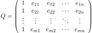
logit(p) =Qβ (7)

where Qis a matrix that includes a constant col-umn of 1, necessary for theβ0of the linear

combi-nation of the values of the regression. Moreover it includes the transpose of the evidence matrix, i.e.

E = (−→e1...−→em). Therefore the matrix will be:

Q=



    

1 e11 e12 · · · e1n 1 e21 e22 · · · e2n

..

. ... ... . .. ...

1 em1 em2 · · · emn 

    

The set of equations in Eq. 7 can be solved us-ing multiple linear regression.

In their general form, the equations of multiple linear regression may be written as (Caron et al.,

1988):

y=Xβ+ε

where:

• y is a column vectorn×1that includes the observed values of the dependent variables

Y1, ..., Yk;

• X is a matrixn×mof the values of the re-gressors that we have observed;

• βis a column vectorm×1of the regression coefficients;

• εis a column vector including the stochastic components that have not been observed and that will not be considered later.

In the caseXis a rectangular and singular matrix, the systemy = Xβ has not a solution. Yet, it is possible to use the principle of the Least Square Estimation. This principle determines the solution

β that minimize the residual norm, i.e.:

b

β= arg minkXβ−yk2 ₍₈₎

This problem can be solved by the Moore-Penrose pseudoinverse X+ (Penrose, 1955). Then, the final equation to determine theβ is

b

β =X+y

It is important to remark that if the inverse matrix exist X+ = X−1 and that X+X and XX+ are symmetric.

For our case, the following equation is valid:

b

β =Q+−−−−−→logit(p)

3.4 Computing Pseudoinverse Matrix with SVD Analysis

matrixQ=UΣVT the pseudo-inverse matrix that minimizes the Eq. 9 is:

Q+=VΣ+UT (9)

The diagonal matrixΣ+_{is a matrixr×robtained}

first transposingΣand then calculating the recip-rocals of the singular value ofΣ. So the diagonal elements of theΣ+are _δ1

1,

1 δ2, ..., ,

1 δr.

We have now our opportunity of using SVD as natural feature selector as we can compute differ-ent approximations of the pseudo-inverse matrix. As we saw in Sec. 2, the algorithm for computing the singular value decomposition can be stopped a different dimensions. We called kthe number of dimensions. As we can obtain different SVD as approximations of the original matrix (Eq. 2), we can define different approximations of :

Q+≈Q+_k =Vn×kΣ+k×kU T k×m

In our experiments we will use different values ofkto explore the benefits of SVD as feature se-lector.

4 Experimental Evaluation

In this section, we want to empirically explore whether our use of SVD feature selection pos-itively affects performances of the probabilistic taxonomy learner. The best way of determining how a taxonomy learner is performing is to see if it can replicate an existing ”taxonomy”. We will ex-periment with the attempt of replicating a portion of WordNet (Miller, 1995). In the experiments, we will address two issues: 1) determining to what extent SVD feature selection affect performances of the taxonomy learner; 2) determining if SVD as unsupervised feature selection is better for the task than some simpler model for taxonomy learn-ing. We will explore the effects on both the flat and theinductiveprobabilistic taxonomy learner.

The rest of the section is organized as follows. In Sec. 4.1 we will describe the experimental set-up in terms of: how we selected the portion of WordNet, the description of the corpus used to ex-tract evidences, a description of the feature space we used, and, finally, the description of a baseline models for taxonomy learning we have used. In Sec. 4.2 we will present the results of the experi-ments in term of performance.

4.1 Experimental Set-up

To completely define the experiments we need to describe some issues: how we defined the taxon-omy to replicate, which corpus we have used to extract evidences for pairs of words, which feature space we used, and, finally, the baseline model we compared our feature selection model against.

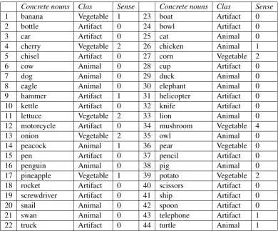
As target taxonomy we selected a portion of WordNet1 (Miller, 1995). Namely, we started from the 44 concrete nouns listed in (McRae et al., 2005) and divided in 3 classes: animal, arti-fact, and vegetable. For sake of comprehension, this set is described in Tab. 2. For each word w, we selected the synset sw that is compliant with

the class it belongs to. We then obtained a setSof synsets (see Tab. 2). We then expanded the set to

S0 adding the siblings (i.e., the coordinate terms) for each synset inS. The setS0 contains 265 co-ordinate terms plus the 44 original concrete nouns. For each element inSwe collected its hyperonym, obtaining the setH. We then removed from the set

H the 4 topmosts: entity,unit,object, andwhole. The setH contains 77 hyperonyms. For the pur-pose of the experiments we both derived from the previous sets a taxonomyT and produced a set of negative examplesT. The two sets have been ob-tained as follows. The taxonomy T is the portion of WordNet implied byO =H∪S0, i.e.,T con-tains all the(s, h) ∈O×O that are in WordNet. On the contrary,T contains all the(s, h)∈O×O

that are not in WordNet. We then have 5108 posi-tive pairs inT and 52892 negative pairs inT.

We then split the setT∪T in two parts, training and testing. As we want to see if it is possible to attach the set S0 to the right hyperonym, the split has been done as follows. We randomly divided the set S0 in two parts Str and Sts, respectively,

of 70% and 30% of the original S0. We then se-lected as trainingTtr all the pairs inT containing

a synset inStrand as testing setTts those pairs of T containing a synset ofSts. For the probabilistic

model,Ttris the initial taxonomy whereasTts∪T

is the unknown set.

As corpus we used theEnglish Web as Corpus (ukWaC) (Ferraresi et al., 2008). This is a web extracted corpus of about 2700000 web pages taining more than 2 billion words. The corpus con-tains documents of different topics such as web, computers, education, public sphere, etc.. It has been largely demonstrated that the web documents

1

Concrete nouns Clas Sense Concrete nouns Clas Sense

1 banana Vegetable 1 23 boat Artifact 0

2 bottle Artifact 0 24 bowl Artifact 0

3 car Artifact 0 25 cat Animal 0

4 cherry Vegetable 2 26 chicken Animal 1

5 chisel Artifact 0 27 corn Vegetable 2

6 cow Animal 0 28 cup Artifact 0

7 dog Animal 0 29 duck Animal 0

8 eagle Animal 0 30 elephant Animal 0

9 hammer Artifact 1 31 helicopter Artifact 0

10 kettle Artifact 0 32 knife Artifact 0

11 lettuce Vegetable 2 33 lion Animal 0

12 motorcycle Artifact 0 34 mushroom Vegetable 4

13 onion Vegetable 2 35 owl Animal 0

14 peacock Animal 1 36 pear Vegetable 0

15 pen Artifact 0 37 pencil Artifact 0

16 penguin Animal 0 38 pig Animal 0

17 pineapple Vegetable 1 39 potato Vegetable 2 18 rocket Artifact 0 40 scissors Artifact 0 19 screwdriver Artifact 0 41 ship Artifact 0

20 snail Animal 0 42 spoon Artifact 0

21 swan Animal 0 43 telephone Artifact 1

22 truck Artifact 0 44 turtle Animal 1

Table 2: Concrete nouns, Classes and senses selected in WordNet

are good models for natural language (Lapata and Keller, 2004).

As the focus of the paper is the analysis of the effect of the SVD feature selection, we used as fea-ture spaces both n-grams and bag-of-words. Out of the T ∪ T, we selected only those pairs that appeared at a distance of at most 3 tokens. Us-ing these 3 tokens, we generated three spaces: (1) 1-gram that contains monograms, (2) 2-gram that contains monograms and bigrams, and (3) the 3-gram space that contains monograms, bigrams, and trigrams. For the purpose of this experiment, we used a reduced stop list as classical stop words as punctuation, parenthesis, the verbto beare very relevant in the context of features for learning a taxonomy.

Finally, we want to describe ourbaseline model for taxonomy learning. This model only contains Heart’s patterns (Hearst, 1992) as features. The feature value is the point-wise mutual information. These features are in some sense the best features for the task as these have been manually selected after a process of corpus analysis. These baseline features are included in our 3-gram model. We can

then compare our best models with this baseline features in order to see if our SVD feature selec-tion model outperforms manual feature selecselec-tion.

4.2 Results

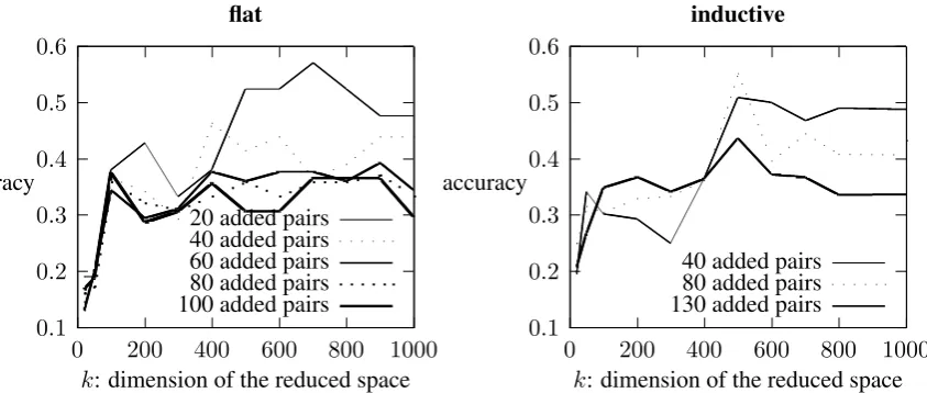
0.1 0.2 0.3 0.4 0.5 0.6

0 200 400 600 800 1000

accuracy

k: dimension of the reduced space flat

20 added pairs 40 added pairs 60 added pairs 80 added pairs 100 added pairs

0.1 0.2 0.3 0.4 0.5 0.6

0 200 400 600 800 1000

accuracy

k: dimension of the reduced space inductive

40 added pairs 80 added pairs 130 added pairs

Figure 1: Accuracy over different cuts of the feature space

0.1 0.2 0.3 0.4 0.5 0.6

0 100 200 300 400 500 600

accuracy

added pairs baseline

1-gram 2-gram 3-gram

Figure 2: Comparison of different feature spaces with k=400

reported for both the flatmodel and theinductive model. The flat algorithm adds one pair at each iteration. Then, we reported curves for each 20 added pairs. Each curve shows that accuracy does not increase after a dimension of k=700. This size of the space is necessary only for the first 20 added pairs. Accuracy keeps increasing to k=700 and then decreases. When we add more pairs, the opti-mal size of the space is around k=200. For the in-ductivemodel we report the accuracies for around 40, 80, 130 added pairs. Here, at each iteration, more than one pair is added. The optimal dimen-sion of the feature space seems to be around 500 as after that value performances decrease or stay stable. SVD feature selection has then a positive effect for both theflatand theinductive probabilis-tic taxonomy learners. This has beneficial effects both on the performances and on the computation time.

added pairs is small. Performances of the three re-duced pairs become similar after 100 added pairs. These experiments show that SVD feature selec-tion has a positive effect on performances as re-sulting models are always better with respect to the baseline.

5 Conclusions and Future Work

We presented a model to naturally introduce SVD feature selection in a probabilistic taxonomy learner. The method is effective as allows the de-signing of better probabilistic taxonomy learners. We still need to explore at least two issues. First, we need to determine whether or not the posi-tive effect of SVD feature selection is preserved in more complex feature spaces such as syntactic feature spaces as those used in (Snow et al., 2006). Second, we need to compare the SVD feature se-lection with other unsupervised feature sese-lection models to determine whether or not this is the best method to use in the case of probabilistic taxon-omy learning.

References

D. Caron, W. Hospital, and P. N. Corey. 1988.

Variance estimation of linear regression coefficients

in complex sampling situation. Sampling Error:

Methodology, Software and Application, pages 688– 694.

D. R. Cox. 1958. The regression analysis of binary sequences. Journal of the Royal Statistical Society. Series B (Methodological), 20(2):215–242.

Scott Deerwester, Susan T. Dumais, George W. Furnas, Thomas K. L, and Richard Harshman. 1990.

In-dexing by latent semantic analysis. Journal of the

American Society for Information Science, 41:391– 407.

A. Ferraresi, E. Zanchetta, M. Baroni, and S. Bernar-dini. 2008. Introducing and evaluating ukwac, a

very large web-derived corpus of english. In In

Proceed-ings of the WAC4 Workshop at LREC 2008, Marrakesh, Morocco.

G. Golub and W. Kahan. 1965. Calculating the singu-lar values and pseudo-inverse of a matrix.Journal of the Society for Industrial and Applied Mathematics, Series B: Numerical Analysis, 2(2):205–224.

Isabelle Guyon and Andr´e Elisseeff. 2003. An intro-duction to variable and feature selection.Journal of Machine Learning Research, 3:1157–1182, March.

Zellig Harris. 1964. Distributional structure. In Jer-rold J. Katz and Jerry A. Fodor, editors,The Philos-ophy of Linguistics, New York. Oxford University Press.

Marti A. Hearst. 1992. Automatic acquisition of

hy-ponyms from large text corpora. InProceedings of

the 15th International Conference on Computational Linguistics (CoLing-92), Nantes, France.

Mirella Lapata and Frank Keller. 2004. The web as a baseline: Evaluating the performance of unsuper-vised web-based models for a range of nlp tasks. InProceedings of the Human Language Technology Conference of the North American Chapter of the Association for Computational Linguistics, Boston, MA.

Bing Liu. 2007. Web Data Mining: Exploring

Hy-perlinks, Contents, and Usage Data. Data-Centric Systems and Applications. Springer.

Bernardo Magnini and Manuela Speranza. 2001.

In-tegrating generic and specialized wordnets. InIn

Proceedings of the Euroconference RANLP 2001, Tzigov Chark, Bulgaria.

K. McRae, G.S. Cree, M.S. Seidenberg, and C. McNor-gan. 2005. Semantic feature production norms for a large set of living and nonliving things. pages 547– 559, Behavioral Research Methods, Instruments, and Computers.

George A. Miller. 1995. WordNet: A lexical

database for English. Communications of the ACM,

38(11):39–41, November.

J. A. Nelder and R. W. M. Wedderburn. 1972. Gener-alized linear models.Journal of the Royal Statistical Society. Series A (General), 135(3):370–384.

Donie O’Sullivan, A. McElligott, and Richard F. E. Sutcliffe. 1995. Augmenting the princeton wordnet

with a domain specific ontology. InProceedings of

the Workshop on Basic Issues in Knowledge Sharing at the 14th International Joint Conference on Artifi-cial Intelligence. Montreal, Canada.

Patrick Pantel and Marco Pennacchiotti. 2006.

Espresso: Leveraging generic patterns for automati-cally harvesting semantic relations. InProceedings of the 21st International Conference on Computa-tional Linguistics and 44th Annual Meeting of the Association for Computational Linguistics, pages 113–120, Sydney, Australia, July. Association for Computational Linguistics.

R. Penrose. 1955. A generalized inverse for matrices. InProc. Cambridge Philosophical Society.

Harold R. Robison. 1970. Computer-detectable

se-mantic structures. Information Storage and

Re-trieval, 6(3):273–288.

Rion Snow, Daniel Jurafsky, and A. Y. Ng. 2006. Se-mantic taxonomy induction from heterogenous