Maximum Likelihood Estimation of Feature Based Distributions

Maximum Likelihood Estimation of Feature-based Distributions

Jeffrey Heinz and Cesar Koirala University of Delaware Newark, Delaware, USA {heinz,koirala}@udel.edu

Abstract

Motivated by recent work in phonotac-tic learning (Hayes and Wilson 2008, Al-bright 2009), this paper shows how to de-fine feature-based probability distributions whose parameters can be provably effi-ciently estimated. The main idea is that these distributions are defined as a prod-uct of simpler distributions (cf. Ghahra-mani and Jordan 1997). One advantage of this framework is it draws attention to what is minimally necessary to describe and learn phonological feature interactions in phonotactic patterns. The “bottom-up” approach adopted here is contrasted with the “top-down” approach in Hayes and Wilson (2008), and it is argued that the bottom-up approach is more analytically transparent.

1 Introduction

The hypothesis that the atomic units of phonology are phonological features, and not segments, is one of the tenets of modern phonology (Jakobson et al., 1952; Chomsky and Halle, 1968). Accord-ing to this hypothesis, segments are essentially epiphenomenal and exist only by virtue of being a shorthand description of a collection of more primitive units—the features. Incorporating this hypothesis into phonological learning models has been the focus of much influential work (Gildea and Jurafsky, 1996; Wilson, 2006; Hayes and Wil-son, 2008; Moreton, 2008; Albright, 2009).

This paper makes three contributions. The first contribution is a framework within which:

1. researchers can choose which statistical in-dependence assumptions to make regarding phonological features;

2. feature systems can be fully integrated into strictly local (McNaughton and Papert, 1971)

(i.e. n-gram models (Jurafsky and Martin, 2008)) and strictly piecewise models (Rogers et al., 2009; Heinz and Rogers, 2010) in order to define families of provably well-formed, feature-based probability distribu-tions that are provably efficiently estimable.

The main idea is to define a family of distribu-tions as the normalized product of simpler distri-butions. Each simpler distribution can be repre-sented by a Probabilistic Deterministic Finite Ac-ceptor (PDFA), and the product of these PDFAs defines the actual distribution. When a family of distributionsFis defined in this way,F may have many fewer parameters than if F is defined over the product PDFA directly. This is because the pa-rameters of the distributions are defined in terms of the factors which combine in predictable ways via the product. Fewer parameters means accurate estimation occurs with less data and, relatedly, the family contains fewer distributions.

This idea is not new. It is explicit in Facto-rial Hidden Markov Models (FHMMs) (Ghahra-mani and Jordan, 1997; Saul and Jordan, 1999), and more recently underlies approaches to de-scribing and inferring regular string transductions (Dreyer et al., 2008; Dreyer and Eisner, 2009). Although HMMs and probabilistic finite-state au-tomata describe the same class of distributions (Vidal et al., 2005a; Vidal et al., 2005b), this paper presents these ideas in formal language-theoretic and automata-theoretic terms because (1) there are no hidden states and is thus simpler than FHMMs, (2) determinstic automata have several desirable properties crucially used here, and (3) PDFAs add probabilities to structure whereas HMMs add structure to probabilities and the authors are more comfortable with the former perspective (for fur-ther discussion, see Vidal et al. (2005a,b)).

strong statistical independence assumption: no two features interact. This is shown to capture ex-actly the intuition that sounds with like features have like distributions. Also, the assumption of non-interacting features is shown to be too strong because like sounds do not have like distributions in actual phonotactic patterns. Four kinds of fea-tural interactions are identified and possible solu-tions are discussed.

Finally, we compare this proposal with Hayes and Wilson (2008). Essentially, the model here represents a “bottom-up” approach whereas theirs is “top-down.” “Top-down” models, which con-sider every set of features as potentially interact-ing in every allowable context, face the difficult problem of searching a vast space and often re-sort to heuristic-based methods, which are diffi-cult to analyze. To illustrate, we suggest that the role played by phonological features in the phono-tactic learner in Hayes and Wilson (2008) is not well-understood. We demonstrate that classes of all segments but one (i.e. the complement classes of single segments) play a significant role, which diminishes the contribution provided by natural classes themselves (i.e. ones made by phonologi-cal features). In contrast, the proposed model here is analytically transparent.

This paper is organized as follows. §2 reviews some background. §3 discusses bigram models and §4 defines feature systems and feature-based distributions. §5 develops a model with a strong independence assumption and §6 discusses feat-ural interaction. §7 dicusses Hayes and Wilson (2008) and§8 concludes.

2 Preliminaries

We start with mostly standard notation. P(A)is the powerset ofA. Σdenotes a finite set of sym-bols and a string over Σ is a finite sequence of these symbols. Σ+ andΣ∗denote all strings over this alphabet of nonzero but finite length, and of any finite length, respectively. A function f with domainAand codomainBis writtenf :A→B. When discussing partial functions, the notation↑ and ↓ indicate for particular arguments whether the function is undefined and defined, respectively. Alanguage L is a subset of Σ∗. Astochastic language D is a probability distribution overΣ∗. The probabilitypof wordwwith respect toDis writtenP r_D(w) =p. Recall that all distributions

Dmust satisfyP_w∈Σ∗P r_D(w) = 1. IfLis

lan-guage thenP rD(L) = P_w∈LP rD(w). Since all distributions in this paper are stochastic languages, we use the two terms interchangeably.

A Probabilistic Deterministic Finite-state Automaton (PDFA) is a tuple

M = hQ,Σ, q0, δ, F, Ti where Q is the state set, Σ is the alphabet, q₀ is the start state, δ is a deterministic transition function, F and T are the final-state and transition probabilities. In particular, T : Q×Σ → R+ andF : Q → R+ such that

for allq∈Q, F(q) +X

σ∈Σ

T(q, σ) = 1. (1)

PDFAs are typically represented as labeled di-rected graphs (e.g.M′in Figure 1).

A PDFA M generates a stochastic language

DM. If it exists, the (unique)pathfor a wordw= a0. . . ak belonging to Σ∗ through a PDFA is a

sequence h(q₀, a₀),(q₁, a₁), . . . ,(q_k, a_k)i, where qi+1 =δ(qi, ai). The probability a PDFA assigns

towis obtained by multiplying the transition prob-abilities with the final probability alongw’s path if it exists, and zero otherwise.

P rDM(w) =

k

Y

i=0

T(qi, ai)

!

·F(qk+1) (2)

ifdˆ(q₀, w)↓and 0 otherwise

A stochastic language isregular deterministic iff there is a PDFA which generates it.

Thestructural componentsof a PDFAMis the deterministic finite-state automata (DFA) given by the states Q, alphabet Σ, transitions δ,and initial state q₀ ofM. By thestructure of a PDFA, we mean its structural components.1 _{Each PDFAM}

defines a family of distributions given by the pos-sible instantiations of T and F satisfying Equa-tion 1. These distribuEqua-tions have at most|Q|·(|Σ|+

1) parameters (since for each state there are|Σ| possible transitions plus the possibility of finality.) These are, for allq ∈ Q andσ ∈ Σ, the proba-bilitiesT(q, σ)andF(q). To make the connection to probability theory, we sometimes write these as P r(σ|q)andP r(#|q), respectively.

We define the product of PDFAs in terms of co-emission probabilities (Vidal et al., 2005a). Let M₁ = hQ₁,Σ₁, q₀₁, δ₁, F₁, T₁i and M₂ = 1_{This is up to the renaming of states so PDFA with}

hQ2,Σ2, q02, δ2, F2, T2i be PDFAs. The proba-bility that σ₁ is emitted from q₁ ∈ Q₁ at the same moment σ₂ is emitted from q₂ ∈ Q₂ is CT(σ1, σ2, q1, q2) =T1(q1, σ1)·T2(q2, σ2). Sim-ilarly, the probability that a word simultaneously ends atq₁ ∈ Q₁and atq₂ ∈ Q₂isCF(q₁, q₂) = F1(q1)·F2(q2).

Definition 1 Thenormalized co-emission product of PDFAs M₁ and M₂ isM = M₁× M₂ =

hQ,Σ, q0, δ, F, Tiwhere

1. Q, q₀, and F are defined in terms of the standard DFA product over the state space Q1×Q2(Hopcroft et al., 2001).

2. Σ = Σ₁×Σ₂

3. For all hq₁, q₂i ∈ Q and hσ₁, σ₂i ∈

Σ, δ(hq₁, q₂i,hσ₁, σ₂i) = hq′₁, q₂′i iff δ1(q1, σ1) =q′1andδ2(q2, σ2) =q2′.2

4. For allhq₁, q₂i ∈Q,

(a) let_PZ(hq₁, q₂i) =CF(hq₁, q₂i) + hσ1,σ2i∈ΣCT(σ1, σ2, q1, q2) be the normalization term; and

(b) F(hq₁, q₂i) = CF(_Zq1,q2); and (c) for allhσ₁, σ₂i ∈Σ,

T(hq1, q2i,hσ1, σ2i) =

CT(hσ1,σ2,q1,q2i)

Z

In other words, the numerators of T and F are defined to be the co-emission probabilities, and division by Z ensures that M defines a well-formed probability distribution.3 The normalized co-emission product effectively adopts a statisti-cal independence assumption between the states ofM₁andM₂. IfS is a list of PDFAs, we write N

Sfor their product (note order of product is ir-relevant up to renaming of the states).

The maximum likelihood (ML) estimation of regular deterministic distributions is a solved problem when the structure of the PDFA is known (Vidal et al., 2005a; Vidal et al., 2005b; de la Higuera, 2010). LetSbe a finite sample of words drawn from a regular deterministic distributionD. The problem is to estimate parametersT andFof

2

Note that restrictingδto cases whenσ1 = σ2obtains the standard definition ofδ=δ1×δ2(Hopcroft et al., 2001). The reason we maintain two alphabets becomes clear in§4.

3_Z(hq

1, q2i)is less than one whenever eitherF1(q1)or F2(q2)are neither zero nor one.

M so that D_M approaches D using the widely-adopted ML criterion (Equation 3).

( ˆT ,Fˆ) = argmax

T,F

Y

w∈S

P rM(w) !

(3)

It is well-known that if D is generated by some PDFAM′with the same structural components as

M, then theML estimate ofS with respect toM guarantees that D_M approachesD as the size of S goes to infinity (Vidal et al., 2005a; Vidal et al., 2005b; de la Higuera, 2010).

Finding the ML estimate of a finite sample S with respect to M is simple provided M is de-terministic with known structural components. In-formally, the corpus is passed through the PDFA, and the paths of each word through the corpus are tracked to obtain counts, which are then normal-ized by state. LetM =hQ,Σ, δ, q₀, F, Tibe the PDFA whose parameters F and T are to be esti-mated. For all statesq ∈ Qand symbolsσ ∈ Σ, The ML estimation of the probability of T(q, σ) is obtained by dividing the number of times this transition is used in parsing the sample S by the number of times stateqis encountered in the pars-ing ofS. Similarly, the ML estimation ofF(q)is obtained by calculating the relative frequency of stateq being final with stateqbeing encountered in the parsing ofS. For both cases, the division is normalizing; i.e. it guarantees that there is a well-formed probability distribution at each state. Fig-ure 1 illustrates the counts obtained for a machine

M with sampleS = {abca}.4 Figure 1 shows a DFA with counts and the PDFA obtained after normalizing these counts.

3 Strictly local distributions

In formal language theory, strictly k-local lan-guages occupy the bottom rung of a subregular hierarchy which makes distinctions on the basis of contiguous subsequences (McNaughton and Pa-pert, 1971; Rogers and Pullum, to appear; Rogers et al., 2009). They are also the categorical coun-terpart to stochastic languages describable withn -gram models (wheren =k) (Garcia et al., 1990; Jurafsky and Martin, 2008). Since stochastic lan-guages are distributions, we refer to strictly k -local stochastic languages as strictlyk-local

distri-4_{Technically,Mis neither a simple DFA or PDFA; rather,}

A : 1 a : 2 b : 1 c:1

A:1/5 a : 2 / 5 b:1/5 c:1/5

M M′

Figure 1:Mshows the counts obtained by parsing it with sampleS={abca}.M′shows the proba-bilities obtained after normalizing those counts.

butions (SLD_k). We illustrate with SLD₂(bigram models) for ease of exposition.

For an alphabet Σ, SL₂ distributions have

(|Σ|+ 1)2 _{parameters. These are, for allσ, τ ∈} Σ∪ {#}, the probabilitiesP r(σ|τ). The proba-bility ofw=σ₁. . . σ_nis given in Equation 4.

P r(w)def

= P r(σ1|#)×P r(σ2|σ1)

×. . .×P r(#|σn) (4)

PDFA representations of SL₂ distributions have the following structure: Q= Σ∪ {#},q₀ = #, and for allq ∈ Q andσ ∈ Σ, it is the case that δ(q, σ) =σ.

As an example, the DFA in Figure 2 provides the structure of PDFAs which recognize SL₂ dis-tributions withΣ ={a, b, c}. Plainly, the param-eters of the model are given by assigning proba-bilities to each transition and to the ending at each state. In fact, for all σ ∈ Σ andτ ∈ Σ∪ {#}, P r(σ | τ) is T(τ, σ) and P r(# | τ) is F(τ). It follows that the probability of a particular path through the model corresponds to Equation 4. The structure of a SL₂ distribution for alphabet Σ is given byMSL2(Σ).

Additionally, given a finite sampleS ⊂Σ∗, the ML estimate of S with respect to the family of distributions describable with MSL2(Σ) is given

by counting the parse ofS throughMSL2(Σ)and

then normalizing as described in§2. This is equiv-alent to the procedure described in Jurafsky and Martin (2008, chap. 4).

4 Feature-based distributions

This section first introduces feature systems. Then it defines feature-based SL₂ distributions which make the strong independence assumption that no two features interact. It explains how to find

b

a c

b

a

c

b

a

c

b

a

c #

a

b

c

Figure 2: MSL2({a, b, c})represents the structure

of SL₂distributions whenΣ ={a, b, c}.

F G

a +

-b + +

c - +

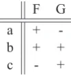
Table 1: An example of a feature system withΣ =

{a, b, c}and two featuresF andG.

the ML estimate of samples with respect to such distributions. This section closes by identifying kinds of featural interactions in phonotactic pat-terns, and discusses how such interactions can be addressed within this framework.

4.1 Feature systems

Assume the elements of the alphabet share prop-erties, called features. For concreteness, let each feature be a total function F : Σ → V_F, where the codomain V_F is a finite set ofvalues. A fi-nite vector of featuresF =hF₁, . . . , F_niis called a feature system. Table 1 provides an example of a feature system with F = hF, Gi and values

VF =VG={+,−}.

We extend the domain of all features F ∈ F to Σ+, so that F(σ₁. . . σ_n) = F(σ₁). . . F(σ_n). For example, using the feature system in Table 1, F(abc) = + +− and G(abc) = −+ +. We also extend the domain of F to all languages: F(L) =∪w∈Lf(w). We also extend the notation so thatF(σ) =hF₁(σ), . . . , F_n(σ)i. For example,

F(c) = h−F,+Gi (feature indices are included for readability).

If, for all arguments ~v,F−1(~v)is nonempty then the feature system is exhaustive. If, for all argu-ments~v such that F−1(~v) is nonempty, it is the case that|F−1(~v)| = 1then the feature system is distinctive. E.g. the feature system in Table 1 in not exhaustive sinceF−1(h−F,−Gi) =∅, but it is distinctive since where F−1 is nonempty, it picks out exactly one element of the alphabet.

Generally, phonological feature systems for a particular language are distinctive but not exhaus-tive. Any feature systemFcan be made exhaustive by adding finitely many symbols to the alphabet (since Fis finite). LetΣ′denote an alphabet ob-tained by adding toΣ the fewest symbols which makeFexhaustive.

Each feature system also defines a set of indi-cator functionsVF= S_f∈F(V_f × {f})with do-mainΣsuch thathv, fi(σ) = 1ifff(σ) = vand

0 otherwise. In the example in Table 1, VF =

{+F,−F,+G,−G} (omitting angle braces for readability). For all f ∈ F, the set VF_f is the

VF restricted to f. So continuing our example,

VFF ={+F,−F}.

4.2 Feature-based distributions

We now define feature-based SL₂distributions un-der the strong independence assumption that no two features interact. For feature system F =

hF1. . . Fni, there arenPDFAs, one for each

fea-ture. The normalized co-emission product of these PDFAs essentially defines the distribution. For each F_i, the structure of its PDFA is given by

MSL2(VF_i). For example, MF = MSL2(VF)

andM_G=MSL2(VG)in figures 3 and 4 illustrate

the finite-state representation of feature-based SL₂ distributions given the feature system in Table 1.5

The states of each machine make distinctions ac-cording to features F and G, respectively. The pa-rameters of these distributions are given by assign-ing probabilities to each transition and to the end-ing at each state (except forP r(#|#)).6

Thus there are2|VF|+P_F∈F|VF_F|2+ 1 pa-rameters for feature-based SL₂ distributions. For example, the feature system in Table 1 defines a distribution with2·4 + 22+ 22+ 1 = 17

param-5

For readability, featural information in the states and transitions is included in these figures. By definition, the states and transitions are only labeled with elements ofVF

andVG, respectively. In this case, that makes the structures of the two machines identical.

6_{It is possible to replaceP r(#|#)with two parameters,}

P r(#|#F)P r(#|#G), but for ease of exposition we do not pursue this further.

-F -F

+ F + F

-F

+ F -F

+ F

#

Figure 3: M_F represents a SL₂distribution with respect to feature F.

-G -G

+ G + G

-G

+ G -G

+ G

#

Figure 4: M_G represents a SL₂distribution with respect to feature G.

eters, which includeP r(#| +F),P r(+F | #), P r(+F |+F),P r(+F | −F), . . . , the G equiva-lents, andP r(#|#). Let SLD2_Fbe the family of distributions given by all possible parameter set-tings (i.e. all possible probability assignments for eachMSL2(VFi)in accordance with Equation 1.)

The normalized co-emission product defines the feature-based distribution. For example, the struc-ture of the product ofM_F andM_G is shown in Figure 5.

As defined, the normalized co-emission product can result in states and transitions that cannot be interpreted by non-exhaustive feature systems. An example of this is in Figure 5 sinceh−F,−Giis not interpretable by the feature system in Table 1. We make the system exhaustive by letting Σ′ =

Σ∪ {d}and settingF(d) =h−F,−Gi.

What is the probability of a given b in the feature-based model? According to the normal-ized co-emission product (Defintion 1), it is

P r(a|b) =P r(h+F,−Gi | h+F,+Gi) =

P r(+F |+F)·P r(−G|+G)

Z whereZ =Z(h+F,+Gi)equals

X

σ∈Σ′

Pr(F(σ)|+F)·Pr(G(σ)|+G)

+ (Pr(#|+F)·Pr(#|+G)

#

+ F , - G + F , - G

+ F , + G + F , + G

-F,+G -F,+G

-F,-G -F,-G

+ F , - G

+ F , + G

-F,+G -F,-G

+ F , - G

+ F , + G

-F,+G -F,-G

+ F , - G

+ F , + G

-F,+G

-F,-G

+ F , - G

+ F , + G

-F,+G -F,-G

Figure 5: The structure of the product ofM_F andM_G.

theP r(σ | τ)is given by Equation 5. First, the normalization term is provided. Let

Z(τ) = X

σ∈Σ 

 Y

1≤i≤n

P r(Fi(σ)|Fi(τ))

 

+ Y

1≤i≤n

P r(#|Fi(τ))

Then

P r(σ|τ) = Q

1≤i≤nP r(Fi(σ)|Fi(τ))

Z(τ) (5)

The probabilities P r(σ | #) and P r(# | τ) are similarly decomposed into featural parameters. Finally, like SL₂distributions, the probability of a word w ∈ Σ∗ is given by Equation 4. We have thus proved the following.

Theorem 1 The parameters of a feature-based SL₂ distribution define a well-formed probability distribution overΣ∗.

ProofIt is sufficient to show for allτ ∈ Σ∪ {#} that P_{σ∈Σ∪{#}}P r(σ | τ) = 1 since in this case, Equation 4 yields a well-formed probability distribution over Σ∗. This follows directly from the definition of the normalized co-emission

product (Definition 1).

The normalized co-emission product adopts a statistical independence assumption, which here is between features since each machine represents a single feature. For example, considerP r(a|b) = P r(h−F,+Gi | h+F,+Gi). The probability P r(h−F,+Gi | h+F,+Gi) cannot be arbitrar-ily different from the probabilitiesP r(−F |+F)

and P r(+G | +G); it is not an independent pa-rameter. In fact, because P r(a | b)is computed directly as the normalized product of parameters P r(−F | +F)andP r(+G | +G), the assump-tion is that the featuresF andGdo not interact. In other words, this model describes exactly the state of affairs one expects if there is no statistical in-teraction between phonological features. In terms of inference, this means if one sound is observed to occur in some context (at least contexts dis-tinguishable by SL₂models), then similar sounds (i.e. those that share many of its featural values) are expected to occur in this context as well.

4.3 ML estimation

The ML estimate of feature-based SL₂ distribu-tions is obtained by counting the parse of a sample through each feature machine, and normalizing the results. This is because the parameters of the dis-tribution are the probabilities on the feature ma-chines, whose product determines the actual dis-tribution. The following theorem follows imme-diately from the PDFA representation of feature-based SL₂distributions.

Theorem 2 LetF=hF₁, . . . F_niand letDbe de-scribed byM = N_1≤i≤nMSL2(VF i). Consider

a finite sampleSdrawn fromD. Then the ML es-timate ofS with respect toSLD2_Fis obtained by finding, for eachF_i∈F, the ML estimate ofF_i(S) with respect toMSL2(VF i).

states of each MSL2(VF_i). By definition, each

MSL2(VF_i) describes a probability distribution

overF_i(Σ∗), as well as a family of distributions. Therefore finding the MLE of S with respect to SLD2_Fmeans finding the MLE estimate ofF_i(S) with respect to eachMSL2(VFi).

Optimizing the ML estimate of F_i(S) for each M_i = MSL2(VFi) means that as |Fi(S)| increases, the estimates TMiˆ and FMiˆ approach the true values TMi and FMi. It follows that as |S| increases, TMˆ and FMˆ approach the true values of TM and FM and consequently D_M

approachesD.

4.4 Discussion

Feature-based models can have significantly fewer parameters than segment-based models. Con-sider binary feature systems, where|VF| = 2|F|. An exhaustive feature system with 10 binary fea-tures describes an alphabet with 1024 symbols. Segment-based bigram models have(1024+1)2=

1,050,625 parameters, but the feature-based one only has 40 + 40 + 1 = 81 parameters! Con-sequently, much less training data is required to accurately estimate the parameters of the model.

Another way of describing this is in terms of ex-pressivity. For given feature system, feature-based SL₂ distributions are a proper subset of SL₂ dis-tributions since, as the the PDFA representations make clear, every feature-based distribution can be described by a segmental bigram model, but not vice versa. The fact that feature-based distribu-tions have potentially far fewer parameters is a re-flection of the restrictive nature of the model. The statistical independence assumption constrains the system in predictable ways. The next section shows exactly what feature-based generalization looks like under these assumptions.

5 Examples

This section demonstrates feature-based gener-alization by comparing it with segment-based generalization, using a small corpus S =

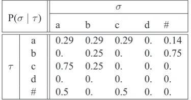
{aaab, caca, acab, cbb} and the feature system in Table 1. Tables 2 and 3 show the results of ML estimation ofSwith respect to segment-based SL₂ distributions (unsmoothed bigram model) and feature-based SL₂ distributions, respectively. Each table shows the P r(σ | τ) for all σ, τ ∈

{a, b, c, d,#} (where F(d) = h−F,−Gi), for

σ P(σ|τ)

a b c d #

a 0.29 0.29 0.29 0. 0.14

b 0. 0.25 0. 0. 0.75

τ c 0.75 0.25 0. 0. 0.

d 0. 0. 0. 0. 0.

# 0.5 0. 0.5 0. 0.

Table 2: ML estimates of parameters of segment-based SL₂distributions.

σ P(σ|τ)

a b c d #

a 0.22 0.43 0.17 0.09 0.09

b 0.32 0.21 0.09 0.13 0.26

τ c 0.60 0.40 0. 0 0.

d 0.33 0.67 0 0 0

# 0.25 0.25 0.25 0.25 0.

Table 3: ML estimates of parameters of feature-based SL₂distributions.

ease of comparison.

Observe the sharp divergence between the two models in certain cells. For example, no words be-gin withbin the sample. Hence the segment-based ML estimates of P r(b | #)is zero. Conversely, the feature-based ML estimate is nonzero because b, likea, is +F, and b, like c, is +G, and both a andcbegin words. Also, notice nonzero probabil-ities are assigned todoccuring afteraandb. This is because F(d) = h−F,−Gi and the following sequences all occur in the corpus: [+F][-F] (ac), [+G][-G] (ca), and [-G][-G] (aa). On the other hand, zero probabilities are assigned todocurring aftercanddbecause there are noccsequences in the corpus and hence the probability of [-F] occur-ing after [-F] is zero.

6 Featural interaction

In many empirical cases of interest, features do interact, which suggests the strong independence assumption is incorrect for modeling phonotactic learning.

There are at least four kinds of featural inter-action. First, different features may be prohib-ited from occuring simultaneously in certain con-texts. As an example of the first type consider the fact that both velars and nasal sounds occur word-initially in English, but the velar nasal may not. Second, specific languages may prohibit dif-ferent features from simultaneously occuring in all contexts. In English, for example, there are syl-labic sounds and obstruents but no sylsyl-labic obstru-ents. Third, different features may be universally incompatible: e.g. no vowels are both [+high] and [+low]. The last type of interaction is that different features may be prohibited from occuring syntag-matically. For example, some languages prohibit voiceless sounds from occuring after nasals.

Although the independence assumption is too strong, it is still useful. First, it allows researchers to quantify the extent to which data can be ex-plained without invoking featural interaction. For example, following Hayes and Wilson (2008), we may be interested in how well human acceptabil-ity judgements collected by Scholes (1966) can be explained if different features do not interact. Af-ter training the feature-based SL₂model on a cor-pus of word initial onsets adapted from the CMU pronouncing dictionary (Hayes and Wilson, 2008, 395-396) and using a standard phonological fea-ture system (Hayes, 2009, chap. 4), it achieves a correlation (Spearman’s r) of 0.751.7 In other words, roughly three quarters of the acceptability judgements are explained without relying on feat-ural interaction (or segments).

Secondly, the incorrect predictions of the model are in principle detectable. For example, recall that English has word-inital velars and nasals, but no word-inital velar nasals. A one-cell chi-squared test can determine whether the observed number of [#N] is significantly below the expected number according to the feature-based distribution, which could lead to a new parameter being adopted to describe the interaction of the [dorsal] and [nasal]

7_{We use the feature chart in Hayes (2009) because it}

con-tains over 150 IPA symbols (and not just English phonemes). Featural combinations not in the chart were assumed to be impossible (e.g. [+high,+low]) and were zeroed out.

features word-initially. The details of these proce-dures are left for future research and are likely to draw from the rich literature on Bayesian networks (Pearl, 1989; Ghahramani, 1998).

More important, however, is this framework al-lows researchers to construct the independence as-sumptions they want into the model in at least two ways. First, universally incompatible features can be excluded. For example, suppose [-F] and [-G] in the feature system in Table 1 are anatomically incompatible like [+low] and [+high]. If desired, they can be excluded from the model essentially by zeroing out any probability mass assigned to such combinations and re-normalizing.

Second, models can be defined where multiple features are permitted to interact. For example, suppose features F and G from Table 1 are em-bedded in a larger feature system. The machine in Figure 5 can be defined to be a factor of the model, and now interactions between F and G will be learned, including syntagmatic ones. The flex-ibility of the framework and the generality of the normalized co-emission product allow researchers to consider feature-based distributions which al-low any two features to interact but which pro-hibit three-feature interactions, or which allow any three features to interact but which prohibit four-feature interactions, or models where only certain features are permitted to interact but not others (perhaps because they belong to the same node in a feature geometry (Clements, 1985; Clements and Hume, 1995).8

7 Hayes and Wilson (2008)

This section introduces the Hayes and Wilson (2008) (henceforth HW) phonotactic learner and shows that the contribution features play in gener-alization is not as clear as previously thought.

HW propose an inductive model which ac-quires a maxent grammar defined by weighted constraints. Each constraint is described as a se-quence of natural classes using phonological fea-tures. The constraint format also allows reference to word boundaries and at most one complement class. (The complement class ofS ⊆ ΣisΣ/S.) For example, the constraint

*#[ˆ -voice,+anterior,+strident][-approximant] means that in word-initial C₁C₂clusters, if C₂is a nasal or obstruent, then C₁must be [s].

8_{Note if all features are permitted to interact, this yields}

Hayes and Wilson maxent models r features & complement classes 0.946 no features & complement classes 0.937 features & no complement classes 0.914 no features & no complement classes 0.885

Table 4: Correlations of different settings versions of HW maxent model with Scholes data.

HW report that the model obtains a correlation (Spearman’sr) of 0.946 with blick test data from Scholes (1966). HW and Albright (2009) attribute this high correlation to the model’s use of natural classes and phonological features. HW also report that when the model is run without features, the grammar obtained scores anrvalue of only 0.885, implying that the gain in correlation is due specif-ically to the use of phonological features.

However, there are two relevant issues. The first is the use of complement classes. If features are not used but complement classes are (in effect only allowing the model to refer to single segments and the complements of single segments, e.g. [t] and [ˆt]) then in fact the grammar obtained scores an r value of 0.936, a result comparable to the one reported.9 Table 4 shows thervalues obtained by the HW learner under different conditions. Note we replicate the main result of r = 0.946 when using both features and complement classes.10

This exercise reveals that phonological features play a smaller role in the HW phonotactic learner than previously thought. Features are helpful, but not as much as complement classes of single seg-ments (though features with complement classes yields the best result by this measure).

The second issue relates to the first: the question of whether additional parameters are worth the gain in empirical coverage. Wilson and Obdeyn (2009) provide an excellent discussion of the model comparison literature and provide a rigor-ous comparative analysis of computational mod-eleling of OCP restrictions. Here we only raise the questions and leave the answers to future research. Compare the HW learners in the first two rows in Table 4. Is the ∼ 0.01 gain in rscore worth the additional parameters which refer to

phono-9

Examination of the output grammar reveals heavy re-liance on the complement class [ˆs], which is not surprising given the discussion of [sC] clusters in HW.

10_{This software is available on Bruce Hayes’ webpage:}

http://www.linguistics.ucla.edu/ people/hayes/Phonotactics/index.htm.

logically natural classes? Also, the feature-based SL₂model in§4 only receives anrscore of 0.751, much lower than the results in Table 4. Yet this model has far fewer parameters not only because the maxent models in Table 4 keep track of tri-grams, but also because of its strong independence assumption. As mentioned, this result is infor-mative because it reveals how much can be ex-plained without featural interaction. In the con-text of model comparison, this particular model provides an inductive baseline against which the utility of additional parameters invoking featural interaction ought to be measured.

8 Conclusion

The current proposal explicitly embeds the Jakob-sonian hypothesis that the primitive unit of phonology is the phonological feature into a phonotactic learning model. While this paper specifically shows how to integrate features into n-gram models to describe feature-based strictly n-local distributions, these techniques can be ap-plied to other regular deterministic distributions, such as strictly k-piecewise models, which de-scribe long-distance dependencies, like the ones found in consonant and vowel harmony (Heinz, to appear; Heinz and Rogers, 2010).

In contrast to models which assume that all features potentially interact, a baseline model was specifically introduced under the assumption that no two features interact. In this way, the “bottom-up” approach to feature-based general-ization shifts the focus of inquiry to the featural interactions necessary (and ultimately sufficient) to describe and learn phonotactic patterns. The framework introduced here shows how researchers can study feature interaction in phonotactic mod-els in a systematic, transparent way.

Acknowledgments

References

Adam Albright. 2009. Feature-based generalisation as a source of gradient acceptability. Phonology, 26(1):9–41.

Noam Chomsky and Morris Halle. 1968. The Sound Pattern of English. Harper & Row, New York.

G.N. Clements and Elizabeth V. Hume. 1995. The internal organization of speech sounds. In John A. Goldsmith, editor, The handbook of phonological theory, chapter 7. Blackwell, Cambridge, MA.

George N. Clements. 1985. The geometry of phono-logical features.Phonology Yearbook, 2:225–252.

Colin de la Higuera. 2010. Grammatical Inference: Learning Automata and Grammars. Cambridge University Press.

Markus Dreyer and Jason Eisner. 2009. Graphical models over multiple strings. InProceedings of the Conference on Empirical Methods in Natural Lan-guage Processing (EMNLP), pages 101–110, Singa-pore, August.

Markus Dreyer, Jason R. Smith, and Jason Eisner. 2008. Latent-variable modeling of string transduc-tions with finite-state methods. InProceedings of the Conference on Empirical Methods in Natural Language Processing (EMNLP), pages 1080–1089, Honolulu, October.

Pedro Garcia, Enrique Vidal, and Jos´e Oncina. 1990. Learning locally testable languages in the strict sense. InProceedings of the Workshop on Algorith-mic Learning Theory, pages 325–338.

Zoubin Ghahramani and Michael I. Jordan. 1997. Fac-torial hidden markov models. Machine Learning, 29(2):245–273.

Zoubin Ghahramani. 1998. Learning dynamic bayesian networks. In Adaptive Processing of Sequences and Data Structures, pages 168–197. Springer-Verlag.

Daniel Gildea and Daniel Jurafsky. 1996. Learn-ing bias and phonological-rule induction. Compu-tational Linguistics, 24(4).

Bruce Hayes and Colin Wilson. 2008. A maximum en-tropy model of phonotactics and phonotactic learn-ing.Linguistic Inquiry, 39:379–440.

Bruce Hayes. 2009. Introductory Phonology. Wiley-Blackwell.

Jeffrey Heinz and James Rogers. 2010. Estimating strictly piecewise distributions. InProceedings of the 48th Annual Meeting of the Association for Com-putational Linguistics, Uppsala, Sweden.

Jeffrey Heinz. to appear. Learning long-distance phonotactics.Linguistic Inquiry, 41(4).

John Hopcroft, Rajeev Motwani, and Jeffrey Ullman. 2001.Introduction to Automata Theory, Languages, and Computation. Boston, MA: Addison-Wesley.

Roman Jakobson, C. Gunnar, M. Fant, and Morris Halle. 1952. Preliminaries to Speech Analysis. MIT Press.

Daniel Jurafsky and James Martin. 2008. Speech and Language Processing: An Introduction to Nat-ural Language Processing, Speech Recognition, and Computational Linguistics. Prentice-Hall, Upper Saddle River, NJ, 2nd edition.

Robert McNaughton and Seymour Papert. 1971. Counter-Free Automata. MIT Press.

Elliot Moreton. 2008. Analytic bias and phonological typology.Phonology, 25(1):83–127.

Judea Pearl. 1989. Probabilistic Reasoning in In-telligent Systems: Networks of Plausible Inference. Morgan Kauffman.

James Rogers and Geoffrey Pullum. to appear. Aural pattern recognition experiments and the subregular hierarchy. Journal of Logic, Language and Infor-mation.

James Rogers, Jeffrey Heinz, Gil Bailey, Matt Edlef-sen, Molly Visscher, David Wellcome, and Sean Wibel. 2009. On languages piecewise testable in the strict sense. InProceedings of the 11th Meeting of the Assocation for Mathematics of Language.

Lawrence K. Saul and Michael I. Jordan. 1999. Mixed memory markov models: Decomposing complex stochastic processes as mixtures of simpler ones. Machine Learning, 37(1):75–87.

Robert J. Scholes. 1966. Phonotactic grammaticality. Mouton, The Hague.

Enrique Vidal, Franck Thollard, Colin de la Higuera, Francisco Casacuberta, and Rafael C. Carrasco. 2005a. Probabilistic finite-state machines-part I. IEEE Transactions on Pattern Analysis and Machine Intelligence, 27(7):1013–1025.

Enrique Vidal, Frank Thollard, Colin de la Higuera, Francisco Casacuberta, and Rafael C. Carrasco. 2005b. Probabilistic finite-state machines-part II. IEEE Transactions on Pattern Analysis and Machine Intelligence, 27(7):1026–1039.

Colin Wilson and Marieke Obdeyn. 2009. Simplifying subsidiary theory: statistical evidence from arabic, muna, shona, and wargamay. Johns Hopkins Uni-versity.