Transport Infrastructure Investment and Transport Sector Productivity on Economic Growth in South Africa (1975 2011)

Transport Infrastructure Investment and

Transport Sector Productivity on

Economic Growth in South Africa

(1975-2011)

CHETENI, PRIVILEDGE

UNIVERSITY OF FORT HARE

12 March 2013

Online at

https://mpra.ub.uni-muenchen.de/53175/

Transport Infrastructure Investment and Transport Sector Productivity on

Economic Growth in South Africa (1975-2011)

Priviledge Cheteni

University of Fort Hare Email: 200909553@ufh.ac.za

Doi:10.5901/mjss.2013.v4n13p761

Abstract

This paper examines the impact of transport infrastructure investment and transport sector productivity on South African economic growth for the period 1975-2011. We use a Vector Error Correction Model and a Bayesian Vector Autoregressive model as empirical tools. The models provide an insight into the dynamic shocks on economic growth through impulse responses. The VECM reveals that economic growth is influenced by inflation, domestic fixed transport investments, and real exchange rate, yet on the BVAR model it was influenced by inflation, domestic fixed transport investments, multi factor productivity, real exchange rate and second period Gross Domestic Product.

Keywords: South Africa, Transport infrastructure, economic growth, transport sector, productivity

1. Introduction

Infrastructure investments have been traditionally viewed as a policy instrument for development in several developing countries. According to the New Growth Path that was launched in 2010 by the Department of Economic Development, infrastructure has been targeted as one of the job drivers in the economy. Presenting the Infrastructure Development Cluster (IDC) briefing in February 2012 the Minister of Transport highlighted the South African government interest to invest in infrastructure and making it a central priority in addressing problems of inequality, poverty and unemployment. Therefore, the government is set to invest over ZAR845 billion in implementing infrastructure projects meant to remedy the distortions of infrastructure such as roads, hospitals, schools, electricity, ports and rail that were created by the apartheid system (IDC, 2012).

There are many macroeconomic studies that have tried to empirically link public infrastructure investments to private sector productivity or to economic growth (Canning & Bennethan, 2000; Aschaeur, 1989). These studies show that; investment in infrastructure contributes positively to economic growth; the impact of infrastructure can have direct or indirect effects on raising marginal product of capital. (Gramlich, 1994; Calderon & Serven, 2004) argued that the direction of causation between public investment and output growth is unclear, leading to ambiguous policy advice. Mittnik and Neumann (2001) argue that public investment can be considered as a factor input to economic growth, but the way it is financed leads to crowding out effects on private investment. Limited research has been done to explore the linkage between infrastructure investment and productivity to economic growth in South Africa (Chakwizira & Mashiri, 2008; Fedderke & Bogetic 2006, Kunaratne, 2001).

This paper therefore seeks to analyse the effects of transport infrastructure investments and transport sector productivity in stimulating economic growth in South Africa for the period 1975-2011. The paper adds another dimension to infrastructure studies by using a Bayesian VAR model to impose restrictions on coefficients of the VAR by assuming that parameters associated with longer lags are more likely to be near zero than coefficients on shorter lags. This is done to overcome the problem of over parameterization and loss of degrees of freedom that are associated with a VAR model.

2. Literature Review

This sections looks into literature review on the effects of infrastructure investments to economic growth.

2.1 Transport Infrastructure in South Africa

are still lagging behind on infrastructure development with the exception of Gauteng, Kwazulu Natal and Cape Town. According to the Department of Transport (2012) most regions are still dealing with a high volume of backlogs in transport projects, this is just one factor explaining lags in certain regions. Bogetic and Fedderke (2006) suggest that the lags in infrastructure development in South Africa may have been a legacy of apartheid and inequalities that exists between the privileged and the poor majority.

However, there have been great improvements in various types of transport facilities like roads and airports partly due to the FIFA World Cup that was hosted in 2010. The government embarked on a number of programmes that led to improvements in transport infrastructure. Airports were upgraded; the OR Tambo International Airport, King Shaka International and the Cape Town Airport were the major beneficiaries of the infrastructure programme. The Gauteng province benefited from the launching of the Gautrain, which was the first speed train in Africa. Nevertheless, all these efforts were not enough to suit the large demand of infrastructure services by the population.

2.2 Transport Infrastructure investments and performance

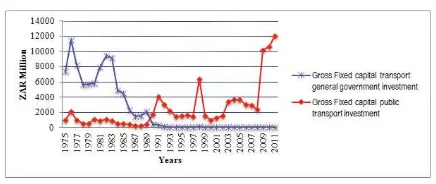
The South African government has been investing in transport infrastructure for many years so as to stimulate growth amongst other target. Figure 1shows fixed capital transport investment since 1975 to 2011.

Figure 1:Gross Fixed Capital Investment (Transport) from 1975-2011

Source:South Africa Reserve Bank, 2012.

The government invested more capital in transport infrastructure in the late 1970s relative to the 1990s. Gross Fixed Capital Formation for the public transport increased by 33.3 percent in 1990s. Robust growth in 1998 and 2010 was a result of the adoption of the Growth, Employment and Redistribution Policies and the Reconstruction and Development Programme amongst others. However, even though the graph shows a decline and stationery growth in general transport investments the total public transport investment was increasing at a steady rate from 2001 to 200. This highlights huge investments that has continued at an accelerated pace until 2011. The total transport investments is at its highest with more than ZAR50 billion invested this far and continues to increase. According to the South Africa Reserve Bank (SARB) Quarterly Bulletin Report as at 2012 the increase in public transport investment since 2008 was mainly due to the roll out of government`s massive infrastructure investment programmes.

2.3 Transport infrastructure performance

In July 2010 the Transport Minister Sibusiso Ndebele was quoted by Engineering News saying that the government would spend ZAR14.5 billion in developing an integrated rapid transport network in the country. The capital expenditure on expansion and replacement of transport infrastructure on a five year plan would cost over ZAR93 Billion with the majority set towards replacement projects on improving efficiency to the already existing infrastructure (Transnet, 2010).

thorough need of refurbishment or repairs. This figure increased in 2007 to more than 60 percent of roads with a life span of more than 25 years old. Road networks in South Africa are shown in Table 1.

Table 1. Length of road infrastructure in South Africa.

Type Length,Km

Surfaced provincial roads 348 100 Surfaced national toll and non-toll roads 15,600 Un proclaimed rural roads 222 900 Metropolitan, Municipal and other 168000

Total 754600

Source:National Treasury, 2008/09

According to the South African Institute of Civil Engineering (SAICE) 2011, many paved metropolitan roads were deteriorating because municipalities lack capacity, skilled resources and funding to efficiently and effectively manage their road networks. Moreover, gravel roads that constitute about 83.3 percent of the road network have been neglected. SAICE (2011) reports that road maintenance delayed for five years increases the repair costs between 6 and 18 times through direct and indirect costs. These costs can be broken down as follows; direct costs are cost of time and fuel wasted driving congested and deteriorated roads and indirect costs include increases to food prices owing to wasted fuel and time spent on deteriorated roads. Also, maintenance backlogs, upgrading and limited capacity hamper the effectiveness of the investments (SAICE, 2011).

In 2010 the King Shaka Airport was commissioned towards the staging of the FIFA World Cup. The airport annual capacity is estimated to be more 7, 5 million passengers. This is set to improve airport efficiencies and handling capacities in addition to the Oliver Tambo and Cape Town International Airports. In 2011 ACSA allocated ZAR17 billion for capital investments for the next five years. These investments would be utilised through ACSA projects. The Port Elizabeth Airport is set to be upgraded so as to improve its capacity. ACSA Airport projects are shown in Table 2.

Table 2. Major Airports Projects.

Project Name Value (US$) Timeframe Status OR Tambo International Airport upgrade and expansion 263 2008-2010 complete King Shaka International Airport 1058 2007-2010 complete Cape Town Airport Upgrade and new terminal 163 2008-2010 complete Cape Town runway Alignment 19 2014 Project announced

Source:Table Generated from Budget Review,2012.

Despite the fact that the rail system of South Africa has been underinvested for over 30 years with many fleets using 1986 technology, it is still competitive in Africa. The South African rail system is still the largest in Africa stretching to about 20 872 km with 8931km electrified. In 2009 the logistic industry handled more 1530 million tons of freight at a cost of ZAR323 billion and covering over 363 billion kilometres (Transnet, 2012). Rail projects to date are shown in Table 3. Transnet unveiled a 5 year expenditure plan of ZAR80, 5 billion for capital expenditure in rail upgrading the capacity of lines through locomotives acquisition, infrastructure maintenances and wagon maintenances (Transnet, 2011). In addition, Transnet would on short term focus in freight line replacement or refurbishment and upgrading rails, signalling and rolling stock due to the backlog (Transnet, 2012).

Table 3. Rail Transport projects

High speed rail 30000 completed Pretoria Rail link 1200 Project approved by the cabinet Freight servicing Ngqura Port N/a completed

Source:Data from Budget Review, 2012

The major ports in South Africa are Durban, Saldanha Bay, Cape Town, Port Elizabeth, Richards Bay and East London. Richards Bay is mainly used as a coal terminal, while the Saldanha Bay and Cape Town ports are used for oil and gas. The ports handle about 96 percent of South Africa`s exports. This has caused further congestion problems at some ports. According to Perkins et al.(2005), cargo demonstrates porting capacity to handle goods and services thereby infrastructure indirectly.

According to Steyn (2010), South Africa ports are said to be substandard in terms of safety, environmental friendliness and efficient maritime transport despite substantial investments. Serious backlogs, under staffing, an ageing workforce, statutory inspections, and a lack of maintenance were identified as problems (Dell & Mneyey, 2008). Transnet Port Terminal (TPT) has committed a capital expenditure worth R33 billion over the next 7 years to stimulate economic growth and efficiencies in ports (Molefe, 2011). According to the Chief Executive of TPT, the main target is to facilitate unconstrained growth, unlock demand and build world class port operations by becoming more efficient. Container hubs like Port Ngqura that was commissioned in 2012 bring substantial benefits to regional economies and cargo owners by reducing total supply chain costs through improved connectivity, improved service levels and, by attracting more shipping lines, leading to increased competition in the shipping industry (Transnet, 2012).

3. Methodology

A number of researchers have explored the relationship between economic growth and public infrastructure. Most studies use a Cobb Douglas function similar to Aschaeur (1989) when estimating public infrastructure in the United States. This approach measures the effect of public infrastructure on output growth and productivity. However, recent studies have used a cost function approach (Nadiri and Mamuneas, 1996; Khanam, 1999). The cost function is prefered because it offers detailed information on cost flexibility of outputs and effects of infrastructure capital on demand for private sector inputs. Furthermore, it is easy to outline the effect of infrastructure investment on firms’ production structure including economies of scale, technical change, demand for employment and private capital stock (Nadiri & Mamuneas, 1996). Most cost functions integrate the generalized Leontief and translog functions. This helps in estimating direct elasticities of substitution which are important in describing patterns and level of complementarity among factors of production.

The cost function is favoured because it avoids the possible correlation between public and private infrastructure (Gillen, 1996). The cost function method has produced mixed results. These differences may arise due to different sets of data or different evaluating methods. Munell (1990) show that the public capital elasticity of output in United States is 0,34 using the production cost. Nadiri and Mamuneas (1991) obtain coefficients between -0.02 to -1.4 using a cost function to measure US manufacturing data. Afraz et. al. (2006) observed that the use of cost function might give a distorted picture on actual services provided by stock considering the degrees of efficiency that characterises past government investments. These problems associated with cost function have led to many researchers favouring physical measures on public infrastructure like the length of road, rail, and kilometres.

Aschauer (1989) using a Cobb Douglas production function found a strong impact of infrastructure capital on aggregate output. A 1 percent increase in public stock of capital increases output by 0, 35 percent. Esterly and Rebelo (1993) using a cross sectional country panel arrived at the same conclusion. On the other hand Holtz (1994) obtains a zero elasticity of output

Kamps (2006) uses a Vector Auto-Regression (VAR) model for a set of OECD countries for the period 1960-2001 and finds statistical significant positive shocks to public infrastructure on output. A Vector Error Correction Model (VECM) was used by Nurudeen and Usman (2010) in analysing government expenditure on infrastructure and economic growth in Nigeria. The study infers that total government capital expenditure has a negative effect on economic growth, however, rising government expenditure on transport and communication leads to an increase in economic growth. Perkins (2005) uses the Auto Regressive Distributed Lag (PSS ARDL) model from Pesaran et.aland discovers that roads infrastructure spending drives economic growth.

between GDP and infrastructure spending. A VAR (Vector autoregressive) model is first formulated for the endogenous variables: Gross Domestic Product (Y), Multi Factor Productivity (MTP), Real Effective Exchange rate (REER), Inflation (INF), Real Domestic Transport fixed investments (RGDI).

3.1 VECM Model specification

Following Sims (1980) the VAR model takes the following form:

= + ( ) + … … … . . … … … (1)

Where is a (n x 1) vector of variables; ( )is a (n x n) polynomial matrix of operator Lwith lag length p, where:

( ) = + + ; … … … (2)

is a (n x 1) vector of constants terms; and is a (n x1) vector of white noise error terms.

Equation (1) is modified to a VECM (vector error correction) to take account of cointegrating relationships:

= + + + … … … (3)

The VECM assumes that in case we have a set of kvariables, we may have co-integrating relationships indicated by rsuch that 0 1.The existence of rco-integrating relationships leads to the hypothesis that :

( ): = … … … (4)

Where is (p x p)DQGȕĮDUH(p x r)matrices of full rank; ( )is a hypothesis of reduced rank ; > 1 represents identification.

The model used in this research is as follows;

All the variables are converted to logarithms so as to remove any trends. The model in (5) assumes the form:

The dependent variable is Y and is on the left side of the equation. The tis the time index.

3.2 BVAR Model specification

In order to have a better insight between the BVAR model that uses prior specifications and VECM model, both models are utilised in this study. Moreover, the study seeks to tests the best model for estimating the impacts of transport infrastructure investments and productivity to economic growth.

According to Todd (1984), Littermen (1986) and Spencer (1993) Bayesian VARs impose restrictions on the coefficients matrix by assuming that parameters associated with longer lags are more likely to be near zero than coefficients on shorter lags. This in turn overcomes the problem of over parameterization and loss of degrees of freedom that are associated with a VAR model (Litterman, 1981). BVAR methods are good in solving shrinkage by imposing restrictions on parameters to reduce the parameter set. The BVAR model is estimated using 2 lags chosen by the Akaike and Hannan-Quinn information criterion. The prior type is Litterman/Minnesota and the residual covariance is set at Full

9$5HVWLPDWH&RHIILFLHQWSULRUVDUHVHWDWDQG/DPEGDȜ1) is set at 0.1 overall tightness of variance of first lag,

LambdaȜ2) set at 0.99 (Relative cross-YDULDEOHZHLJKW)ROORZLQJ.D\LGDODDQG.DUOVVRQ/DPEGDȜ3) is set

at 1 (Lag decay).

Consider a case where k = 2. In this case the number of co-integrating vectors maybe (r =0, 1). A bivariate vector is in form of _{= ( , )} for t =1……T . This can be expressed as a VAR as follows:

= + + … … … . … … … … (8)

Where is assumed to be white noise error term. The function = _{( )}, where is a square

coefficient matrix. The absence of rank restrictions on matrix implies is a stationary vector. The Minnesota prior means and variance are of this form:

~ (1, ) and ~ (0, ……… (9)

Where denotes coefficients associated with lagged variables in each equation in a VAR, represents any other coefficients. The prior variances and represents uncertainty about the prior means _{= 1}and _{= 0}.

3.3 Co-integration

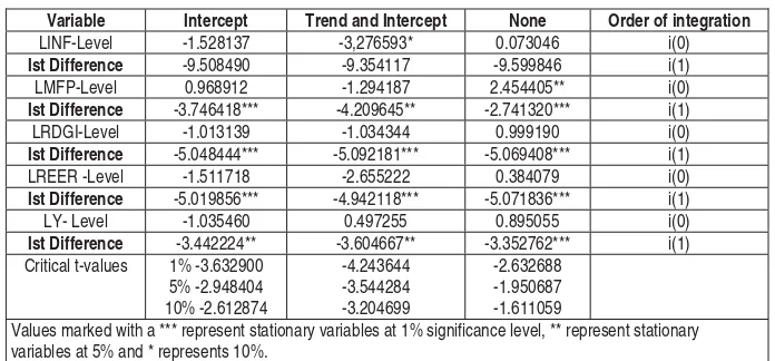
The study firstly examined the properties of stationarity in the time series. The Augmented Dickey Fuller (ADF) Tests was utilised for this process to test the unit root of the variables under study. Results are shown in Table 4. The series is

) 5 .( ...

5 4

3 2

0 l t j t j t j t j t j t

t MTP REER INF RGDI GDP e

Y

–

–

–

–

–

–

) 7 .( ...

5 4

3 2

0 l t j t j t j t j t j t

stationery at first difference i(0).

Table 4. Stationarity Tests

Variable Intercept Trend and Intercept None Order of integration

LINF-Level -1.528137 -3,276593* 0.073046 i(0)

Ist Difference -9.508490 -9.354117 -9.599846 i(1)

LMFP-Level 0.968912 -1.294187 2.454405** i(0)

Ist Difference -3.746418*** -4.209645** -2.741320*** i(1)

LRDGI-Level -1.013139 -1.034344 0.999190 i(0)

Ist Difference -5.048444*** -5.092181*** -5.069408*** i(1)

LREER -Level -1.511718 -2.655222 0.384079 i(0)

Ist Difference -5.019856*** -4.942118*** -5.071836*** i(1)

LY- Level -1.035460 0.497255 0.895055 i(0)

Ist Difference -3.442224** -3.604667** -3.352762*** i(1)

Critical t-values 1% -3.632900 5% -2.948404 10% -2.612874

-4.243644 -3.544284 -3.204699

-2.632688 -1.950687 -1.611059

Values marked with a *** represent stationary variables at 1% significance level, ** represent stationary variables at 5% and * represents 10%.

The lags specifications were determined using E-Views 8 that selected a maximum of 2 lag orders that were deemed to be enough. The five criterions shown in Table 5 recommended LR, FPE, AIC, SC and HQ hence lag 2 was chosen to estimate the VECM Model.

Table 5. Lag Selection

Lag LogL LR FPE AIC SC

0 64.75440 NA 1.84e-08 -3.621479 -3.394735 1 225.5755 263.1617 5.00e-12 -11.85306 -10.49260* 2 267.9163 56.45440* 1.95e-12* -12.90402* -10.40984 3 285.3391 17.95080 4.23e-12 -12.44479 -8.816897 4 316.6213 22.75072 5.89e-12 -12.82554 -8.063921 * indicates lag order selected by the criterion

LR: sequential modified LR test statistic (each test at 5% Level) FPE: Final prediction error

AIC: Akaike information criterion SC: Schwarz information criterion HQ: Hannan-Quinn information criterion

The next stage was the examination of co-integration. This was done to establish a long run relationship among variables. The VAR equation with klags is the same as equation (1) and the Johansen test requires the VAR to be transformed into a Vector Error Correction Model of the form as equation (3)

Where the ‘long run matrix’ is

( ) … … … (11)

is a vector of intercept that may enter the system in the cointergrating vector or as trend is a set of coefficient matrices, is a non zero matrix of elements (Enders, 1995). If =0 then VAR represented in equation (1) is valid in first differences. However if ȆWKHQWKHV\VWHPKDVDQHUURUFRUUHFWLRQPRGHO9(&0ZKLFKLPSOLHVWKDW

= + … … … . (12)

When testing for co integration the rank of Ȇis supposed to be equal to the number of co integrating vectors, r, and is affected by how the Ȇ0enters the system. If r=0 there is no co-integrating vectors. The Johansen co-integration

uses two tests to determine the co-integrated vectors;

( ) = ln (1 ) … … … . . (13)

( + 1) = (1 ) … … … . (14)

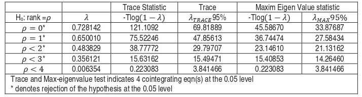
the Maximum Eigen value test and Trace test. The Maxima Eigen value statistic tests the null hypothesis of r co-integrating relations against the alternative r+1co-integrating relation for r=0,1, n-1.The Trace statistic checks the null hypothesis of rco-integrating relations against the alternative of n where n is the number of variables in a system for r=0, 1 ... n-1.

Table 6. Trace and Eigenvalue Tests

Trace Statistic Trace Maxim Eigen Value statistic Ho: rank = -Tlog(1 ) 95% -Tlog(1 ) 95%

= 0* 0.728142 121.1092 69.81889 45.58670 33.87687

= 1* 0.650010 75.52246 47.85613 36.74474 27.58434

< 2* 0.483829 38.77772 29.79707 23.14610 21.13162

< 3* 0.356121 15.63162 15.49471 15.40853 14.26460

< 4 0.006354 0.223083 3.841466 0.223083 3.841466

Trace and Max-eigenvalue test indicates 4 cointegrating eqn(s) at the 0.05 level * denotes rejection of the hypothesis at the 0.05 level

The results of the integration tests on Trace and Eigen Maximum indicated that the time series variables are co-integrated with 4 vectors. The results are consistent with the findings of Fedderke et al.(2006) and Kularatne (2001) among others. Results are presented in Table 6. Therefore, a long run equilibrium relationship exists among all variables in the model. Both the Trace and Eigen test rejects the null hypothesis of no co integrating vectors (r= 0) at the 5% level when tested against the hypothesis of one co-integrating vector (r =1) since the test statistic of 121, 1 is greater than the critical value of 69, 8 for the trace statistic and the same for Eigen were the test statistic is 45, 5 which is greater than the critical value of 33.8. Both tests show that there are 4 integrated vectors in the system.

4. Data

Annual data on real GDP, Real Effective Exchange Rate (REER), Inflation (INF), Real Gross Domestic Fixed Investment (Rm 2005 Prices) and Multi Factor Productivity (lndex 2005) from South Africa for the period of 1975-2011 are used in this study. Data of Real Gross Domestic Fixed Investment and Multi factor productivity was gathered from the National Productivity Institute of South Africa; data of GDP, inflation and real exchange rate was sourced from Quantec Database, World Bank Database and the South Africa Reserve Bank.

In employing the determinants of GDP the aim is to use proxies that have been used in previous literature in order to find a basis of comparison. Among scholars who have used a number of proxies too measure impacts on economic growth, Bakare (2011) used a nominal exchange rate and inflation to measure the impacts of investment to economic growth in Nigeria. Therefore, this study adopts real effective exchange rate (REER) and inflation as a variable. Following Kemmerling and Stephan (2008) study on determinants and productivity of regional transport investments, this study adopts the variable Multi Factor Productivity that captures both labour and capital in production. Solow (1956) posits that an increase in accumulation in physical capital constitute to the growth of the economy. Therefore, real domestic fixed transport investment is proxied as physical capital.

5. Diagnostic Tests

The Jarque Bera test of normality was used in testing normality of the residuals in the VECM model as shown inTable 7.

The Jarque Bera test for all variables jointly accepted the null hypothesis of normal distribution. The LM test was used to test serial correlation. The LM probability results are more than five percent therefore we accept the null that there is no serial correlation at Lag 2.

Table 7. Diagnostic Tests

Test Null Hyphothesis T Statistic Probability

6. Results

6.1 VECM Results

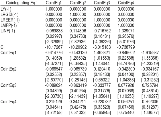
The long run impacts on growth and productivity are shown in Table 8.The table shows that variables in co-integration equation 1 RGDI and MFP have a positive relationship with GDP in the long run, with REER and INF being negative. Co-integration equation 4 suggests that only GDP is significant in explaining the Multi Factor Productivity because thet statistic is over 2. The results are consistent with (Marriotti, 2002) findings that a higher inflation rate leads to a decline in investments as capital goods become expensive, hence, leading to a lower economic growth rate. Therefore, it can be noted that higher inflation and exchange rate have a huge effect in investments decisions in the long run. Moreover, inflation has a huge influence to Multi Factor productivity because when it is high most firms resort to retrenchment which in turn reduces productivity leading to a decline in economic growth. The adjustment coefficient on CointEq1 for the GDP is negative and quite rapid at 61 percent a year, yet for MFP in CointEq 4 is positive and quite small at 6 percent and insignificant. However, the adjustment of GDP is quite higher compared to the 50 percent that was recorded by Fedderke (2004) using the ARDL method. This shows that the speed of adjustment after a deviation from equilibrium is 61 percent and corrected within one year as the variable moves towards restoring equilibrium. Hence, this shows that there is limited pressure on GDP to restore to long run equilibrium wherever there is a disturbance in economy.

Table 8. Long run VECM results

Cointegrating Eq: CointEq1 CointEq2 CointEq3 CointEq4 LY(-1) 1.000000 0.000000 0.000000 0.000000 LRGDI(-1) 0.000000 1.000000 0.000000 0.000000 LREER(-1) 0.000000 0.000000 1.000000 0.000000 LMFP(-1) 0.000000 0.000000 0.000000 1.000000 LINF(-1) -0.069833 0.114396 -0.716762 -1.339071 (0.02997) (0.34733) (0.16431) (0.26676) [-2.32989] [ 0.32936] [-4.36226] [-5.01976] C -10.17267 -10.20902 -3.015183 -0.738799

CointEq1 -0.614776 -0.443120 1.462821 -0.846602 -1.915987 (0.14059) (1.28682) (1.01553) (0.22588) (1.55368) [-4.37271] [-0.34435] [ 1.44044] [-3.74796] [-1.23319] CointEq2 -0.066547 -0.065739 0.120410 -0.042800 -0.934167 (0.02552) (0.23357) (0.18433) (0.04100) (0.28201) [-2.60770] [-0.28145] [ 0.65322] [-1.04388] [-3.31252] CointEq3 -0.089624 -0.863419 -0.333777 0.077928 0.725794 (0.04399) (0.40264) (0.31776) (0.07068) (0.48614) [-2.03730] [-2.14439] [-1.05041] [ 1.10258] [ 1.49297] CointEq4 0.219129 0.344211 -0.220732 0.056251 0.762006 (0.04641) (0.42478) (0.33523) (0.07456) (0.51287) [ 4.72158] [ 0.81033] [-0.65845] [ 0.75440] [ 1.48577]

The VECM results suggested evidence of error correction as shown in Table 9.The relationship between GDP and Multi factor productivity is positive meaning that there may be some form of causality between the two variables in the short run. An increase of 1 percent in Multi factor productivity in the first period is expected to lead to an increase in GDP of 0.09 percent in period one and 0.13 percent in period two. This is supported by economic theory which states that as you increase labour supply, output tends to increase. Snowdon and Vane (2005) note that by increasing capital–labour ratio an economy will experience diminishing marginal productivity. This maybe particular true for South Africa were investment declined in early 1990s and the government concentrated on creating more employment leading to a high labour-capital ratio. Furthermore, research done by Coe et. al.(1997) indicated that total factor productivity of developing countries is positively and significant related to imports in capital investments. The decline in capital investment since 1975 to late 2000s might have influenced productivity in the transport sector.

Variable Coefficient T -statistic Probability C 0.006892 1.144406 0.00602*** LY (-1) (-2) 0.192826 -0.072509 1.050727 -0.27860 0.18352 0.26026 LREER (-1) (-2) -0.015955 0.022314 -0.409271 0.539190 0.03899*** 0.04138*** LRGDI (-1) (-2) -0.068837 0.025344 2.45528 1.104397 0.02804*** 0.02295*** LINF (-1) (2) 0.129746 0.064561 4.151019 3.560212 0.03126*** 0.01813*** LMFP (-1) (-2) 0.095996 0.131421 0.627545 1.357216 0.15297 0.09683*** ***Significant at 5 percent level.

Moreover, the results show that Inflation (LINF), Real Exchange Rate (REER) and Domestic Fixed Transport Investments are significant for a 2 year period. The results are in support of (Perkins, Fedderke & Luiz, 2005) findings that infrastructure seems to have a direct and indirect effect on economic growth in South Africa. However, the results argue that there is one direction relationship between real domestic fixed transport investments and economic growth. A high GDP rate does not necessarily lead to a higher investment in transport or vice versa. An increase of 1 percent in LRGDI is expected to increase GDP by 0.06 percent in the first period and 0.02 percent in the second period. This shows that the positive impact of LRGDI to GDP is eroded as years go by.

Although an increase in investment is expected to increase GDP it does not necessarily mean that an increase in GDP would yield the same effect. However, the results are in support of other international findings (Aschauer, 1989; Munnell, 1992; Lau and Sin, 1997; Arora & Bhundia, 2003) which state that investments have a positive impact to economic growth.

The VECM results show that a decline or increase in exchange rate/inflation has an effect on growth. These findings are in support of Fedderke (2005) who notes that macroeconomic stability contributes to higher investments spending directly through raising the expected returns on projects and indirectly through reducing uncertainty to expectations. Further, Mariotti (2002) highlighted that reduction in inflation has a net benefit to economic growth in South Africa. This is supported by the Philips curve which proved that hyperinflation reduces output, and inflation of less than 2 percent per annum stimulates domestic output. du Plessis (2004) is of the view that is difficult to control exchange rate in an attempt to connect the Rand volatility and economic growth. Hence, exchange rate has a negative impact in period one and a positive impact in period two.

Table 10. BVAR results

Variable Coefficient T -statistic Probability

C 4.229651 3.09996 0.0049 LY (-1) (-2) 0.495574 0.070526 7.55270 1.56327 0.06562 0.04511*** LREER (-1) (-2) -0.029054 -0.050833 -2.17839 -0.66239 0.01334*** 0.00778*** LRGDI (-1) (-2) 0.023092 0.005270 2.75967 0.96266 0.00837*** 0.00547*** LINF (-1) (2) -0.018863 -0.006361 -2.38690 -1.39198 0.00790*** 0.00457*** LMFP (-1) (-2) 0.036628 0.014202 1.21181 0.47052 0.03023*** 0.03018***

***Significant at 5 percent level.

eroded as years go by. In Table 10 it is quite clear that the results for the BVAR method are more robust and supported by a number of economics literature. All the variables have a huge influence to economic growth and productivity. Economically it is expected that one period GDP effects would be felt in the 2 period due to time lags. Therefore, the BVAR results are more robust than the VECM results this can be shown through the Impulse responses graphs.

6.2 Impulse response

6.2.1 VECM

The impulse response show dynamic responses of GDP (LY) to one period shock to the system over a 10 year period. A one period shock to LINF, LREER, LRDGI and LMFP reduces GDP (LY) by almost 12 percent in a 4 year period then the impact continues negative but at a decreasing rate. The GDP has a negative relationship with all variables except LREER at period 6. Moreover, a negative shock decreases GDP at faster rate compared to a positive shock. The impulse responses report that economic growth has a negative relationship with multifactor productivity, real domestic investment and inflation in the long run. As more labour and capital is increased their impacts to GDP will be negative due to diminishing returns. This is shown in Figure 2.

6.2.2 BVAR

The impulses responses of a BVAR are somewhat totally different to the VECM. A one period shock to LRGDI, LREER, LINF and LMFP would lead to a negative shock to GDP for 2 periods then suddenly the impact subsidises. A negative shock to inflation (LINF) and positive shock to LRGDI, LREER, LMFP after a two year period leads to a positive and steady GDP. The impulse responses show that a positive shock to all determinants of GDP except inflation would lead to a positive growth of over 20 percent in a 10 year period. This is in line with expected prior whereby a negative shock to inflation is not expected to have a serious impact in reducing GDP and positive shocks to exchange rate, multi factor productivity, domestic fixed investment are expected to improve GDP. The BVAR impulses are shown in Figure 3.

-.016 -.012 -.008 -.004 .000 .004 .008 .012 .016 .020

1 2 3 4 5 6 7 8 9 10

LY LRGDI LREER

LMFP LINF V ECM

Re sponse of LY t o Chole sk y O ne S.D. I nnova t ions

-.005 .000 .005 .010 .015 .020 .025 .030

1 2 3 4 5 6 7 8 9 10

LY LRGDI LREER

LMFP LINF BV AR

7. Conclusion and Recommendations

The paper examined the impacts of transport infrastructure investment and transport sector productivity on growth in South Africa (1975-2011) using a VECM and BVAR model. The broad results suggests that: Inflation, real exchange rate and real domestic gross fixed transport investment have a positive impact to economic growth according to the VECM model; and inflation real exchange rate, multi-factor productivity, real domestic fixed transport investments, GDP in period 2 have a positive impact to economic growth and productivity.

To stimulate growth and productivity through infrastructure investment, the government should, therefore, increase funding at the same time maintain a low inflation rate. This can be achieved by monitoring fiscal and monetary policies to maintain growth rate of the aggregate demand in combination with public infrastructure policy and other policies as well. Development and management of infrastructure and the provision of public services is indeed the only way to meet the growing infrastructure needs in South Africa. Hence, the current route taken by the government to increase infrastructure investment should be supported so as to improve infrastructure growth in the long run and provide supporting services to sectors such as the Manufacturing and Mining. Moreover, the labour unrests currently persistent in the mining sector have a huge effect on Multi Factor productivity and may lead to a decline in economic growth as shown by the weakening rand in international markets and an increase in inflation rate. Hence, it is imperative that the government should address labour concerns at the earliest time possible to avoid a decline in economic growth and productivity that would be mainly felt by the poor majority.

References

ACSA. 2012. Integrated Annual Report.

Andren. T. (2007). Econometrics. Thomas Andren and Ventus Publishing Aps.

Arora, V., & Bhundia, A. (2003). Potential output and total factor productivity growth in post-Apartheid South Africa. IMF Working Paper No. 03/178. Washington, USA.

Aschauer, D. A. (1989). Is public expenditure productive? Journal of Monetary Economics, 23, 177-200.

Aschauer, D. A. (2000). Do states optimise? Public capital and economic growth. The Annals of Regional Science, 34, 343-363. Barro, R. (1990). Government Spending in a Simple Model of Endogenous Growth. Journal of Political Economy, 98(5), 102-.125.

Berechman, Y., & Banister, D. (2006). Transport investments and the promotion of economic growth. Journal of Transport Geography, 9(2001), 209-218.

Bogetic, Z., & Fedderke, J. W. (2006). International benchmarking of South Africa`s infrastructure performance. World Bank Policy Research Working Paper No. 3830.

Brock, W.A., Dechert W.D., Scheinkman J.A & LeBaron, B. (1996). A Test for independence based on correlation Dimension. Econometric Review, 15, 197-235.

Business Monitor International. (2011). Infrastructure Report. Business Monitor International Ltd: South Africa.

Calderon, C., & Serven, L. (2004). The Effects of Infrastructure Development On Growth and Income Distribution. Central Bank of Chile. Working Papers No 270.

Canning, D., & Bennathan, E. (2000). The social rate of return on infrastructure investments. World Bank Research Project, RPO 680-89, Washington, D.C.

Chakwizira, J., & Mashri, M. (2008). The contribution of transport governance to socio-economic development in South Africa. CSIR Working Paper.

Cipamba Wa Cipamba, P. (2013). The export-output relationship in South Africa: An empirical investigation. ERSA Working paper No. 355. Coe, D, T., Elhanan, H., & Alexander W. H. (1997). North-South R&D Spillovers. Economic Journal, 107, (440), 134–49.

Department of Transport. (2012). The Infrastructure development Cluster Media Briefing. [ONLINE] Available at: http://www.transport.gov.za/LinkClick.aspx?fileticket=c9GgQjVKdPc%3D&.... [Accessed 17 October 12]

Department of Transport.( 2012). Transnet Limited Annual Report 2009. [ONLINE] Available at: http://www.transport.gov.za/. [Accessed 17 October 12].

Department of Transport. (2010). Moving South Africa.

Dell. Y., & Mneney, R. (2008). Enhancing the Port Infrastructure Maintenance System of the Transnet National Ports Authority in South Africa. Watermill Working Paper Series 2008, no. 13.

du Plessis, S. A. (2004). Stretching the South African Business Cycle. Economic Modelling, 21(1), 685-701. Enders, W. (1995). Applied econometric time series. New York: Wiley.

Easterly, W., & Rebelo, S. (1993). Fiscal policy and Economic Growth: An empirical investigation, Journal of Monetary Economics, 32, 417-458. Fedderke, J. W. (2004). Investment in Fixed Capital Stock: testing for the impact of sectorial and systematic uncertainty. Oxford Bulletin of

Economics and Statistics. 66(2),165-187.

Fedderke, J.W. (2005). Technology, human capital and growth. Invited address to the G-20 meeting on economic growth in Pretoria, South Africa on 4-5 August.

Fedderke, W., & Bogetic, Z. (2006). Infrastructure and Growth in South Africa: Direct and Indirect Productivity Impacts of 19 Infrastructure Measures. World Bank Working Paper: 3989.

32(1), 39

Gramlich, E. M. (1994). Infrastructure investment: A review essay. Journal of Economic Literature, 32, 1176-1196. Gujarati, D. (2004). Basic Econometrics. Fourth Edition. The Mcgraw Hill Companies.

Holtz, E. D. (1994). Public Sector Capital and the Productivity Puzzle, Review of Economics and Statistics, 76: 12-21.

Jiang, B.Q. (2001). A Review of Studies on the Relationship between Transport Infrastructures. Investments and Economic Growth, Vancouver, British Columbia.

Kadiyala, K, R., & Karlsson, S. (1997). Numerical methods for estimation and inference in Bayesian VAR-models. Journal of Applied Econometrics, 12, 99-132.

Kamps, C. (2006). Is there a lack of public capital in the European Union? EIB Papers.

Kemmerling, A., & Stephan, A. (2008). The politico-economic determinants and productivity effects of regional transport investment in Europe. EIB PAPERS, 13, 36-61.

Khanam, B. R. (1996). Highway Infrastructure Capital and Productivity Growth: Evidence from the Canadian Goods-Producing Sector. Logistics and Transportation Review, 3(1), 251-268.

Kularatne, C. (2001). An examination of the Impact of financial deepening on long run economic growth: An application of a VECM structure to a middle income country context. ESRA Working Paper No.24. University of Witwatersrand.

Kularatne, C. (2002). An Examination of the Impact of Financial Deepening on Long-Run Economic Growth: An Application of a VECM Structure to a Middle-Income Country Context. South African Journal of Economics, 70(4), 647-87.

Lau, S. H. P., & Sin, C. Y. (1997). Public infrastructure and economic growth: time-series properties and evidence. Economic Record, 73, 125-135.

Litterman, R. B. (1981). A Bayesian Procedure for Forecasting with Vector Auto regression. Working Paper. Federal Reserve Bank of Minneapolis.

Litterman, R. B. (1986). Forecasting with a Bayesian Vector Autoregression-Five Years of Experience. Journal of Business and Economics Statistics, 4(1), 24-38.

Mariotti, M. (2002). An examination of the Impact of Economic Policy on long run economic growth: An application of a VECM structure to a middle income context. ERSA Working paper, University of Witwatersrand.

Mittnik, S., & Neumann, T. (2001). Dynamic effects of public investment: Vector autoregressive evidence from six industrialized countries. Empirical Economics, 26(2), 429-446.

Molefe, B. (2011). Transnet, Outlook and Financials. [ONLINE] Available at: http://www.transnet.net/BusinessWithUs/MDS/External %20Magazine%20-%20Final.pdf. [Accessed 24 October 12].

Munnell, A. H. (1990). Why has productivity growth declined? Productivity and public investment. New England Economic Review, 3-22. Munnell, A. H. (1992). Infrastructure investment and economic growth, Journal of Economic Perspectives, 6(4), 189-198.

Nadiri, M.I., & Mamuneas, T. P. (1991). The Effects of Public Infrastructure and R&D Capital on the Cost Structure and Performance of U.S. Manufacturing Industries. National Bureau of Economic Research, Working Paper No. 3887.

Nadiri, M. I., & Mamuneas, T. P. (1996). Contribution of Highway Capital to Industry and National Productivity Growth.

Nurudeen, A., & Usman, A. (2010). Government Expenditure and Economic Growth In Nigeria, 1970-2008: A Disaggregated Analysis. Business and Economics Journal, 2010 (4), 1-11.

Perkins, P., Fedderke, J.W., & Luiz, J.M. 2005. An Analysis of Economic Infrastructure Investment in South Africa. South African Journal of Economics, 73(2): 211-28.

[49] Pritchett, L. 1996. Where Has All the Eduation Gone? The World Bank, Policy Research Working Paper No. 1581. Quantec. (2012). South African Standardised Industry Database, Quantec Research. Available from http://www.easydata.co.za/ Rothman, P. (1992).The comparative power of the tr test against simple threshold models. Journal of Applied Econometrics, 7, 187-195. SAICE. (2011). Infrastructure Report Card for South Africa.

SANRAL. (2012). Various Reports, Available online:

http://www.nra.co.za/live/content.php?Category_ID=72 [Accessed 20 June 2012) Sims, C.A.( 1980). Macroeconomics and Reality. Econometrica, 48, 1-48.

Snowdon, B., & Vane, H. R. (2005). Modern Macroeconomics: Its Origins, Development and Current State. Edward Elgar Publishing Inc. Massachusetts, USA.

Solow, R. (1956). A contribution to the theory of economic growth. Quarterly Journal of Economics, 50, 65-94.

South African Reserve Bank. (2012).Annual Economic Report. Various issues. Online: http://www.resbank.co.za/Publications /QuarterlyBulletins /Pages/QuarterlyBulletins-Home.aspx

Steyn. (2010). National Planning Commission. [ONLINE] Available at: http://www.npconline.co.za/pebble.asp?relid=184. [Accessed 18 October 12].

Spencer, D. E. (1993). Developing a Bayesian Vector Autoregression. International Journal of Forecasting. 9, 407-421.

The South African National Roads Agency SOC Limited (SANRAL). (2012). Strategic Plan 2012/2013 to 2016/2017. [ONLINE] Available at: http://www.nra.co.za. [Accessed 17 October 12].

Todd, R. M. (1984). Improving economic forecasting with Bayesian Vector Autoregression. Quarterly Review, Federal Reserve of Minneapolis. 18-19.