Novel Optimized Cross Layer Design with Maximum Weighted Capacity Based Resource Allocation for AMC/HARQ Wireless Networks

(1)

Novel Optimized Cross-Layer Design with Maximum

Weighted Capacity Based Resource Allocation for

AMC/HARQ Wireless Networks

Reham A. El-Mayet1_{, Hesham M. El-Badawy}2_{, Salwa H. Elramly}1

1_{Electronic and Communication Department, Ain Shams University, Cairo, Egypt;}2_{National Telecommunication Institute, Cairo,} Egypt.

Email: [email protected], [email protected], [email protected]

Received November 24th_,_{2012; revised January 6}th_{, 2013; accepted January 19}th_{, 2013}

Copyright © 2013 Reham A. El-Mayet et al. This is an open access article distributed under the Creative Commons Attribution Li-cense, which permits unrestricted use, distribution, and reproduction in any medium, provided the original work is properly cited.

ABSTRACT

To provide quality-of service (QoS) guarantees for heterogeneous applications, most recent wireless communications technologies and standards combine the error-correcting capability of hybrid automatic repeat request (HARQ) schemes at the data link layer (DLL) with the adaptation ability of the adaptive modulation and coding (AMC) modes at the physical layer (PHY) layer. This paper aims to investigate the aggregated system capacity as well as the breakdown of this capacity for different ACM modes in each HARQ scheme. This investigation was done by using maximum weighted capacity (MWC) resource allocation at the PHY layer in conjunction with a novel packet error rate (PER)- based scheduling at the medium access control (MAC) layer. As a result, the dominant AMC mode corresponding to channel SNR was available.

Keywords: AMC; Cross-Layer Design; HARQ; Nakagami-m Fading Channel; QoS

1. Introduction

In order to enhance the throughput of the wireless com-munication system, link adaptation (LA) technologies are considered not only at the physical layer, but also at the upper-protocol-layers such as data link layer when de-signing the wireless networks. LA technologies use the instantaneous channel state information (CSI) to adap-tively control the data transmission of wireless channel, maintain constant transmission power to reduce the in-terference of other users and satisfy different business’ needs, and save resources to improve overall throughput for the system. In addition, the adaptive system can eas-ily provide services with different qualities, such as higher information transmission rate, lower packet error rate, and higher spectral efficiency. LA technologies mainly include adaptive modulation and coding (AMC) at the physical layer (PHY) and hybrid automatic repeat request (HARQ) at the data link layer (DLL). The AMC schemes can be used to match transmission rates to time- varying channel, in order to obtain maximum throughput and improve spectral efficiency [1]. Cross-layer design (CLD) which combines AMC and HARQ is extensively studied in order to match the transmission rates to time-

varying wireless communication channel conditions [2]. HARQ provides a good tackling technique to solve the tradeoff between channel coding and packet retransmis-sion. It is a well suited solution to enforce the link quality at the medium access control (MAC) layer in wireless environments, and has been adopted in some towards-4G standards (3GPP LTE Release 8, for instance) [3]. It also can be considered as a combination of forward error cor-rection (FEC) and automatic repeat request (ARQ) which is used to improve reliability [1].

A major concern in data communication is how to con-trol transmission errors caused by channel noise so that error-free data can be delivered to the user. A solution to this problem is using HARQ schemes:

(2)

re-ceiver, similar to standard ARQ [4]. The disadvantage of the type I HARQ scheme is that once the code rate is fixed, all parity bits for error correction are transmitted even if they are not all needed, thus reducing the channel use efficiency [5].

Type-II HARQ, it’s an incremental redundancy (IR) HARQ. It considers the time selective property of the wireless channels. At first transmission, the data packet has no or little redundancy. If it fails, each retransmission includes additional redundancy bits from channel en-coder; the redundancy is increased in the repeated trans-mission of the same packet. Thus, retranstrans-mission of type-II HARQ only uses the information bits that have not been transmitted in the previous transmissions. If all the channel coded information bits have been transmitted, then the channel code will be retransmitted. When the decoder has received the information packet, it combines all the information packets together to decode. The re-transmission packet could not decode alone, it could be decoded only if it was combined together with the pre-vious transmitted information packet [2].

Type-III HARQ, it also an IR scheme but it uses the concept of self-decodable codes; it can be combined with the error data stored and then decoded. The retransmis-sion uses the puncture matrix which is complementary with the puncture matrix for the first transmission. Every puncture matrix has the same code rate and the same error-correction ability [2]. At the receiver, if a frame is detected to be in error, it is stored and a negative ac-knowledgement (NACK) is fed back. Upon arrival of the retransmission, the receiver attempts to decode the sec-ond transmission of the frame. If the decoding is suc-cessful, an ACK is fed back; otherwise the frame is stored and combines all the packets together to decode. The retransmission will continue until the decoding is successful or maximum number of transmission has reached [6].

HARQ in 3GPP Long Term Evolution (LTE), both LTE and LTE-Advanced (LTE-A) use HARQ. In LTE, HARQ reordering is done in the radio link control (RLC) layer. So, it operates into different modes: the unac-knowledged mode (without ARQ) or in acunac-knowledged mode (with active ARQ). In LTE-A, HARQ is very similar to HARQ in LTE, only small adaptations have been done to cope with the change in the supported bandwidth since LTE-A is supposed to support band-width up to 100 MHz [7].

In wireless networking, quality of service (QoS) plays a crucial role in performance measurement. There are four main schemes that are carried out for dynamic sub-carrier and power allocation to different OFDM systems users, which allow a flexible multiuser access and en-hancement of the multiuser diversity [2]: maximum

ca-pacity based resource allocation, proportional fairness based resource allocation, adaptive subcarrier and power allocation in OFDM based on maximizing utility and maximum weighted capacity (MWC) based resource allo-cation.

The AMC/HARQ CLD concept has been proposed in many literatures such as [1,2,4,6]. In [1], the performance of type I, II, III HARQ with AMC over Nakagami-m fading channel was analyzed, a closed form expression of PER and average spectral efficiency were derived and the conditional probability density function of signal-to- noise ratio (SNR) was calculated using Marcov model. In [2], the HARQ (type-II, type-III) was applied to the cross-layer framework in order to satisfy the prescribed delay and PER constraints at LL. In [4], Jaume Ramis had proposed an analytical link level queuing model to formulate a cross-layer design conceived as a constrained optimization problem to exploit the joint impact on QoS performance of both AMC at the PHY layer and HARQ- chase combining based-error control at the DLC-layer. Feijn Shi studied the joint design of type-III HARQ pro-tocol at the data link layer and AMC scheme at the PHY layer through closed-form expressions for throughput, average delay and packet loss rate in [6]. Cross-layer scheduling techniques for multiuser OFDM system were introduced in [8,9] by Nan Zhou: in [8], a packet batch based cross-layer scheduling scheme was proposed. This scheme considers the differences between the batches in the same queue, so it is more flexible and efficient than conventional queue based scheduling. In [9], cross-layer resource allocations based on MWC technique and delay satisfaction (DS) scheduling scheme in the downlink multiuser OFDM system were proposed. The current paper will try to investigate the CLD and its enhance-ments for OFDM based wireless networks. Differently from the previously mentioned publications, the current paper introduces another vision for CLD in both uplink and downlink multiuser OFDM system by considering the packet error rate (PER) as well as the SNR con-straints on the overall performance.

In this paper, based on the AMC/HARQ cross-layer design, the system capacity was investigated for different SNR of OFDM channels for different HARQ schemes. Also, a novel PER based data scheduling technique based on MWC resource allocation was proposed.

In Section 2, the system model is presented. Sub-car-rier and power allocation are presented in Section 3. PER based data scheduling is presented in Section 4. Numeri-cal results and analysis are shown in Section 5. Finally, Section 6 concludes this paper.

2. System Model

(3)

[image:3.595.309.536.546.735.2]

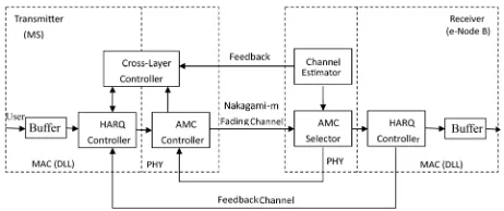
Figure 1, showing the most important blocks involved in the transmission and reception processes for a single user. The HARQ protocol with AMC is used over the Naka-gami-m fading channel, the channel gain is assumed to be constant during the transmission of one frame, and it varies during the transmission of the next frame. Also, the channel is assumed to support QoS-guaranteed traffic characterized by a packet error rate (PER) and a prede-termined acceptable link layer PER Ploss. The processing

unit at the data link layer is a packet of fixed size, and the processing unit at the physical layer is a frame made of a variable number of packets that depends on the transmis-sion mode (TM) selected by the AMC scheme. The re-ceiving buffer can accurately detect the received SNR and decide the next modulation scheme, then feedback channel state message to the source node. On the other hand, if the destination node cannot decode the received data packet correctly, it feeds back NACK signaling to the source node, otherwise, it feeds back acknowledge (ACK) signaling, and the transmission of all signaling messages are assumed to be error free, the maximum number of retransmissions is denoted Rmax.

2.1. Channel Modeling

This paper adopts The Nakagami-m channel model. .The probability density function (pdf) of the received SNR γ, is given by [2]:

 

_{ }

1 e 1

2

m m m

m

m P

m

  

 



   __ _  



 m (1)

where, γ is the instantaneous received SNR, and

 

: E

   is the average received SNR; m is the Naka- gami fading parameter (m ≥ 1/2).

 

1 is the

0

: m e

m t

  

 

_

t

gamma function.

[image:3.595.57.288.612.709.2]

2.2. Combining AMC with HARQ Schemes Given γ in the previous channel model, the objective of AMC is to select a suitable TM to maximize the data rate

Figure 1. Single link between a single-antenna transmitter (MS) and a single-antenna receiver (e-Node B).

while maintaining a prescribed PER Ploss.

To combine the AMC at PHY and HARQ schemes at LL, only finite delays could be afforded. So, the maxi-mum number of the transmission of one packet Rmax

could be determined by dividing the maximum allowable system delay over the round trip delay required for each transmission. If a packet is still erroneous after Rmax

transmissions, it will be dropped, packet loss is declared. So, acceptable Ploss should be predetermined [2].

To simplify the design, the following approximate in-stantaneous PER expression is used [1,2,6]:

 

1, _ _ if 0

PER

e M , if

pM

M g

M p

a  _M

  

 



  

 





(2)

here, M is the mode index to identify the AMC mode. The parameters aM,gM and pM are mode-dependent

parameters, which are listed in Tables 1 and 2 for packet length Np = 1080 bits. These parameters are obtained by

fitting Equation (2) to the exact PER [10]. This expres-sion is used to approximate the PER, when the convolu-tional code is used. Tables 1 and 2 show the values of these parameters for HARQ-type II and HARQ-type III respectively [2].

In the following Tables 1 and 2, the index r in pa-rameters ar,M and gr,M, represents the number of

retrans-mission. r = 0, 1, 2, 3 represent the first, second, third and fourth transmission. M = 1 - 6 represent the AMC mode.

For the type-I HARQ, PER of each transmission is the same as the first transmission of type-II, III HARQ. So, the parameters a0,M and g0,M are the PER curve fitting

parameters of type-I HARQ for each AMC mode. The expression of the PER for type-I HARQ is given by:

 0,

0, e M

g

M M

P a   (3) Table 1. Transmission modes for type II HARQ [2].

Type-II Mode 1 Mode 2 Mode 3 Mode 4 Mode 4 Mode 5 Modulation BPSK QPSK QPSK 16-QAM 16-QAM 64-QAM

Code Rate 1/2 1/2 3/4 3/4 3/4 3/4

Rn(bits/sym.) 0.5 1 1.5 3 3 4.5

a0,n 1525.9 424.06 27.429 126.88 133.27 60.556

g0,n 6.0354 2.6532 0.8483 0.4446 0.2430 0.0553

a1,n 0.2608 163.34 1940 99.5411 359.118 172.666

g1,n 3.5497 1.5291 2.4865 0.4986 0.4812 0.1242

a2,n 13.134 401.49 149.355 178.966 224.796 56.311

g2,n 7.8735 3.1401 2.4442 0.5944 1.5547 0.1485

a3,n 1.0888 1807.2 46.2931 207.57 1064 40.7133

(4)

[image:4.595.57.285.112.327.2]

Table 2. Transmission modes for type III HARQ [2].

Type-III Mode 1 Mode 2 Mode 3 Mode 4 Mode 4 Mode 5 Modulation BPSK QPSK QPSK 16-QAM 16-QAM64-QAM

Code Rate 1/2 1/2 3/4 3/4 3/4 3/4

Rn

(bits/sym.) 0.5 1 1.5 3 3 4.5

a0,n 1525.9 424.06 27.429 126.88 133.27 60.556

g0,n 6.0354 2.6532 0.8483 0.4446 0.2430 0.0553

a1,n 0.2608 0.96857 0.017374 1.2538 0.0273 9.1637

g1,n 3.5497 1.5291 0.61528 0.4569 0.1341 0.14264

a2,n 13.134 1.4037 877.64 1.8815 0.5573 0.0762

g2,n 7.8735 2.6295 3.4533 0.5538 0.4107 0.0909

a3,n 1.0888 0.07827 0.11309 1.0951 1.4994 0.5364

g3,n 8.7707 2.0908 1.1894 0.5096 0.5258 0.1286

Based on the parameters in the Tables 1 and 2, the PER curves for the type-II, III HARQ can be calculated from:    0, 1, max max max 0, 0, 1, 1, e e M R M g M M g

R M R M

P a P a         

 (4)

P0,M is the PER for the first transmission, PR_max1,M is the PER for the Rmaxth transmission, the index M is the

AMC mode.

Equation (5) must be valid, in order to satisfy that the PER is lower than the packet loss probability Ploss after

the Rmax transmissions at LL:

 





0, max1, max max max max 0, 1, 1

loss : target max

e

M R M

g g

R R

M R M

R

a a

P P R

                        

(5)

Then, the average PER for each mode is given by:







max

PER , e gM

M  R a_M   (6)

where,













max max max

max 0, 1,

0, 1,

max

max R

M M R

M R M

M

a R a a

g g g R R M        

 (7)

For the type-I HARQ, in order to satisfy the PER requirement at LL, max max

l1oss

R R

M

P P , then we get  max

loss t 1 arget : R M

P P P (8)

2.3. Different AMC Mode Interval Calculation The parameter Ptarget(Rmax) is a key parameter transferred

from LL to PHY. Ptarget(Rmax) transfers the PER

con-straint Ploss and the time delay requirement Rmax to PHY,

M, M 1



   _

 

1 1 d , , M M i M

P M P

m m m m m   _              _ _ _     



M      e

(10)

where,



_,



_: m1 t_d is complementary in com-

x t

m x    t

 

_

plete Gamma function.

3. Subcarrier and Power Allocation for the

Downlink

By considering a downlink OFDM system with U users, it’s assumed that each subcarrier is occupied by only one user [11]. With cross-layer optimization, the QoS infor-mation is transferred from the traffic controller at the MAC layer to the subcarrier, and power controller at the PHY layer for resource allocation. Then, the resource allocation results are fed-back to the traffic controller in the base station for scheduling of the data to be sent out in each slot [8].

(5)

Let, Ωu denotes the index set of subcarriers allocated to

user u . Let pu,n be the power allocated to

user u on subcarrier n; (n ∊Ωu). hu,nis the corresponding

channel gain. No is the power spectral density of Additive

White Gaussian Noise (AWGN). By assuming perfect channel estimation, the achievable data rate of user u on subcarrier n is expressed as [9]:



u1, ,U





, log 12 ,

u n u n u n

B

R p

N 

  _,



(11)

where, 2 , , u n u n o h N B N

 

(12)

is the channel-to-noise power ratio for user u on subcar-rier n.

Therefore, the total data rate of user u is given by:

, u u n R R 





_{u n}

(13) A resource allocation scheme had been proposed in [2], to maximize the weighted sum of all users’ capacity J, i.e., to maximize

1

U

u u u

J W R





(14)

Subject to: _, _, _total

1

0,

u

U

u n u n

u n

p p

 



 

P





and,

i j i j

    





1 2 U  1, 2, ,N ,

   

where, Wu denotes the weight for user u, which is

evalu-ated based on the cross-layer optimization criteria. So it indicates the QoS information for user u, and is obtained from the result of data scheduling at the MAC layer as will be investigated in Section 4 and Ptotal denotes the

total power.

The optimization process is divided into two stages namely, subcarrier allocation and power allocation. 3.1. Optimal MWC Based Subcarrier Allocation For simplicity, by assuming uniform power allocation across all subcarriers, i.e., each subcarrier is allocated a power p P total N. Optimal subcarrier allocation leads to

the maximum cost function, which is denoted by Jmax. If

an arbitrary subcarrier n allocated to user u

with optimal subcarrier allocation is now reassigned to user s, let



u1, ,U



J denote the resulting cost function. The difference between the two cost functions is given by [9]:

max u u n, s s n, 0

J JW R W R 

(15)

Substituting (11) into (15), we have









2 2 , log 1 log 1 , s n u

s u n

p W W p    



(16)

which implies that, with optimal subcarrier allocation, subcarrier n should be allocated to user u rather than us-ers if Equation (16) is satisfied. However, it is prohibi-tively complex to perform optimal subcarrier allocation with a large number of subcarriers. Therefore, a subop-timal scheme is desired.

 Suboptimal MWC based subcarrier allocation

Intuitively, to maximize the cost function in Equation (14), a larger weight demands a higher data rate. Let Ru/Wu denote the Rate-to-Weight Ratio (RWR) and

as-suming uniform power allocation across all subcarriers. Then, the following suboptimal subcarrier allocation scheme is employed, where the user with the lowest RWR is allowed to pick subcarriers in each of iteration [9]:

1) Initialization:

a) Set Ru =0,   u for all u , sort Wu

in the descending order, and let



u 1, ,



 



1, 2, ,U



L  N denote the set of unallocated subcarriers.

For u = 1 to U:

b) If u m, u n, ( ,m n L m n ;  ), assign subcarrier m

to user u, i.e., add subcarrier m to Ωu. Remove subcarrier

m from L. Update Ru according to Equation (5).

2) Find the minimum Ru/Wu , and repeat 1

b) for the corresponding user u.



k 1, ,

 U



3) Repeat 2) until L .

3.2. Optimal MWC Based Power Allocation Following subcarrier allocation, the optimal power allo-cation for each user can be obtained by using the La-grange multiplier, i.e., (14) can be rewritten as:

, Total

1 1 u

U U

u u u n

u u n

J W R  p P

  

 

    

 



 

(17)

Subject to 1 u , Tot and pu,n ≥ 0. Let- U

u n u n p P

 

al

ting  J p_{u n}_, 0, the optimal solution for pu,nis given by:

 



,



,

1

Total

1 , ,

max size of 1 1 ,0 j u n

u n U

i u

U

i q i q u n

W p W P              _           



 

i



(18)

Consider users j and u (j u, 



1, ,U ), and subcarrier m ∊Ωj and n ∊Ωu are two arbitrary subcarriers allocated

to users j and u, respectively. By  J p_{u n}_,   J p_{i m}_, 0, we can drive:









, , , , , 1 1

u n j m j m i

j j m u n u n,

p W W p      

(6)

1) If Wj/Wu = 1, from (19) it can be derived that:

,

, ,

,

j m u n j m u n

j m u n

p p  

 



  (20)

Equation (20) implies that with equal weight, the sub-carrier with a better channel gain is allocated more power, which is the same result as water-filling [12].

2) If W W_j _u 1, we have:

,

, ,

,

j m u n j m u n

j m u n

p p  

 



  (21)

Equation (21) implies that the subcarrier correspond-ing to the user with a higher weight is allocated more power than the case using water-filling.

4. Packet Error Rate Based Data Scheduling

After receiving the resource allocation results from the PHY layer, which indicates the amount of data allowed for each user, the MAC layer performs scheduling for each batch of data to be sent out. This paper proposes a novel scheduling scheme, which assigns the weight de-pending on the average PER in each ACM mode, after the intervals of different ACM modes are calculated from Equation (9).

The weight Wu denotes the weight of the batch of user

u corresponding to the ACM mode Mi, which is given by:

1 _{for PER} _{PER max}

1

for PER PER max

u

i

U W

T

 

 _

  

 



(22)

where, Ti is the total number of users in ACM mode i,

and  1.

Equation (22) gives higher priority to the user whose batch of data has the maximum PER.

To give the higher priority to the user whose batch of data has the minimum PER, the following equation may be used:

1 _{for PER} _{PER max}

1

for PER PER max

u

i

U W

T

 

 _

  

 



(23)

5. Numerical Results and Analysis

In order to investigate the proposed cross-layer optimiza-tion scheme, numerical results will be deduced for HARQ schemes over a Nakagami-m fading channel. The data unit is assumed to be one frame, and each frame contains a fixed number of symbols. The receiving buffer can accurately detect the received γ and decides the next

modulation scheme, then feedback channel state message to the source node; on the other hand, if the destination node cannot decode the received data packet correctly, it feeds back NACK signaling.

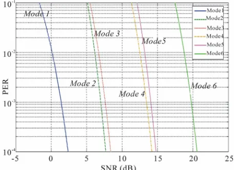
[image:6.595.309.538.350.516.2]

5.1. SNR Margins for Different HARQ Modes In order that, the different modulation and coding schemes is assessed in the case of having only the AWGN. So, Figure 2 presents the obtained probability of PER against the apparent SNR for different AMC modes.

Figures 2 and 3 show the case of having different SNR margins to sustain the PER at a certain range. The obtained results in Figures 2 and 3 are in consistence with those published in many references as [1,2].

The retransmission technique depends on the used HARQ scheme. Also, it is assumed that the transmissions of all signaling messages are assumed to be error free, maximum number of retransmissions, Rmax = 4 and the

ACM modes M = 6.

[image:6.595.310.536.547.715.2]

Figure 2. Different ACM modes for type II HARQ.

(7)

5.2. Effect of Proposed PER Scheduling Criteria on the System Capacity

This paper employs the proposed MWC based resource allocation at the PHY layer and the PER based schedul-ing at the MAC layer for consistency. It considers a LTE system listed in [13], with U = 100 users, a total transmit power of Ptotal = 1 W, a total bandwidth of B = 10 MHz,

subcarrier width of 15 KHz, physical source block code of 180 KHz bandwidth and 50 available Physical Re-source Block (PRB). The power spectral density of AWGN is N0 = −80 dBW/Hz [9] and δ in Equations (22)

and (23) is taken to be 0.8.

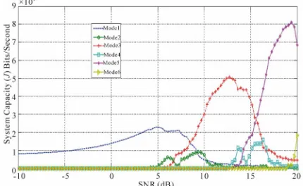
Figures 4 and 5 show the obtained throughput for each mode by deploying the minimum PER using Equation (23) after running different number of iterations with different HARQ techniques. Whereas, Figures 6 and 7 show the obtained throughput for each mode by deploy-ing the maximum PER usdeploy-ing Equation (22) after runndeploy-ing different number of iterations with different HARQ tech-niques.

[image:7.595.315.530.385.517.2]

So, it may be noticed that, the PER maximum as well as the minimum margins are closely estimating the vali-

[image:7.595.62.283.385.515.2]

Figure 4. Average SNR against system capacity (J) HARQ type II-minimum PER.

Figure 5. Average SNR against system capacity (J) HARQ type III-minimum PER.

dation range for each AMC mode separately. This may be explained as a result of having good and stable CLD optimization for different AMC modes with different HARQ.

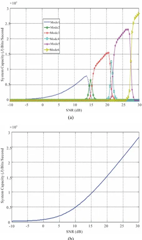
5.3. Effect of Service Requests on HARQ-Type III

Figures 8-10, are investigating the effect of having more customers talking on the same Enhanced e-NodeB site and contenting upon the available throughput.

So, these figures show that by increasing the number of customers, it’s noticed that there’s a steady increase in the required SNR to achieve the same throughput. This may be explained by that the system will be more starv-ing to the power in order to overwhelm the existstarv-ing in-terference which arises from the existing customers. 5.4. LTE System Capacity with Proposed CLD

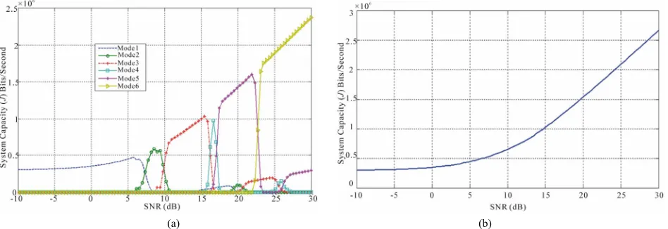
Based PER Scheduling

In Figures 11-14, it is shown that for LTE system parameters, HARQ type III will have much better performance (aggregated throughput) than that of HARQ type II. This

[image:7.595.61.282.557.706.2]

Figure 6. Average SNR against system capacity (J) HARQ type II-maximum PER.

[image:7.595.317.532.559.707.2]

(8)

[image:8.595.310.537.95.478.2]

may be explained by that the HARQ type III will have higher coding gain so, the obtained throughput is im-proved and can be achieved in lower SNR (compared to HARQ type II required SNR).

[image:8.595.61.285.152.301.2]

Figure 8. Average SNR against system capacity (J) K = 100- HARQ type III.

Figure 9. Average SNR against system capacity (J) K = 200- HARQ type III.

Figure 10. Average SNR against system capacity (J) K = 300-HARQ type III.

(a)

(b)

Figure 11. (a) Average SNR against system capacity (J) for each mode in LTE system with proposed maximum PER based scheduling-HARQ type II; (b) Average SNR against aggregated system capacity (J) in LTE system with pro-posed maximum PER based scheduling-HARQ type II.

6. Conclusion

[image:8.595.58.284.342.499.2] [image:8.595.59.285.543.708.2]

(9)

(a) (b)

Figure 12. (a) Average SNR against system capacity (J) for each mode in LTE system with proposed minimum PER based scheduling-HARQ type II; (b) Average SNR against aggregated system capacity (J) in LTE system with proposed minimum PER based scheduling-HARQ type II.

(a) (b)

Figure 13. (a) Average SNR against system capacity (J) for each mode in LTE system with proposed maximum PER based scheduling-HARQ type III; (b) Average SNR against aggregated system capacity (J) for each mode in LTE system with pro-posed maximum PER based scheduling-HARQ type III.

(a) (b)

Figure 14. (a) Average SNR against system capacity (J) for each mode in LTE system with proposed minimum PER based scheduling-HARQ type III; (b) Average SNR against aggregated system capacity in LTE system with proposed minimum

ER based scheduling-HARQ type III. P

[image:9.595.71.528.97.266.2] [image:9.595.70.528.318.482.2] [image:9.595.62.536.534.697.2]

(10)

REFERENCES

[1] C.-Q. Dai, Y. Rao, L. Jiang, Q.-B. Chen and Q. Huang, “Cross-Layer Design of Combining HARQ with Adap- tive Modulation and Coding for Nakagami-m Fading Channels,” Journal of Communications, Academy Pub- lisher, Vol. 7, No. 6, 2012, pp. 458-463.

[2] C. C. Li, L. L. Xu and D. F. Yuan, “Performance Analy- sis and Comparison of HARQ Schemes in Cross Layer Design,” Fourth International Conference on Communica- tions and Networking in China, Ji’nan, 26-28August 2009, pp. 1-5.

[3] S. Marcille, P. Ciblat and C. J. Le Martret, “A Cross- Layer HARQ scheme Robust to Imperfect Feedback,” 2012 Conference Record of the Forty Sixth Asilomar Con- ference on Signals, Systems and Computers, 4-7 Novem- ber 2012, pp. 143-147.

[4] J. Ramis, G. Femenias, F. Riera-Palou and L. Carrasco, “Cross-Layer Optimization of Adaptive Multi-Rate Wire- less Networks Using Truncated Chase Combining HARQ,”

Global Telecommunications Conference, Palma de Mal- lorca, 6-10 December 2010, pp. 1-6.

[5] S. Kallel and D. Haccoun, “Generalized Type II Hybrid ARQ Scheme Using Punctured Convolutional Coding,”

IEEE Transactions on Communications, Vol. 38, No. 11, 1990, pp. 1938-1946. doi:10.1109/26.61474

[6] F. Shi, D. Yuan and L. Xu, “Performance Analysis of Type-III HARQ Scheme in Cross-Layer Design for Quos- Guaranteed Traffic,” International Workshop on Cross Layer Design,Ji’nan,20-21 September 2007, pp.133-137. doi:10.1109/IWCLD.2007.4379055

[7] A. M. Cipriano, P. Gagneuri, G. Vivier and S. Sezginer, “Overview of ARQ and HARQ in Beyond 3G System,”

IEEE 21st_{International Symposium on Personal}_,_Indoor

and Mobile Radio Communications Workshops, Colombes, 26-30 September 2010, pp. 424-429.

[8] N. Zhou, X. Zhu, Y. Huang and H. Lin, “Novel Batch Dependant Cross-Layer Scheduling for Multiuser OFDM Systems,” IEEE International Conference, Beijing, 19-23 May 2008, pp. 3878-3882.

[9] N. Zhou, X. Zhu and Y. Huang, “Cross-Layer Optimiza- tion with Guaranteed QoS for Wireless Multiuser OFDM Systems,” IEEE 18th International Symposium on Per- sonal, Indoor and Mobile Radio Communications, Athens, 3-7 September 2007, pp. 1-5.

[10] X. Wang, Q. Liu and G. B. Giannakis, “Analyzing and Optimizing Adaptive Modulation Coding Jointly with ARQ for QoS-Guaranteed Traffic,” IEEE Transactions on Vehicular Technology, Vol. 56, No. 2, 2007, pp. 710- 720. doi:10.1109/TVT.2007.891465

[11] Z. Shen, J. G. Andrews and B. L. Evans, “Adaptive Re- source Allocation in Multiuser OFDM Systems with Pro- portional Rate Constraints,” IEEE Transactions on Wire- less Communications, Vol. 4, No. 6, 2005, pp. 2726-2737. doi:10.1109/TWC.2005.858010

[12] T. M. Cover and J. A. Thomas, “Elements of Information Theory,” Wiley, New York, 1991.

doi:10.1002/0471200611

[13] “3GPP Long Term Evolution: System Overview, Product Development and Test Challenges,” Agilent Technology, 2009.