Bayesian modelling of skewness and kurtosis with two piece scale and shape transformations

Munich Personal RePEc Archive

Bayesian modelling of skewness and

kurtosis with two-piece scale and shape

transformations

Rubio, Francisco Javier and Steel, Mark F. J.

University of Warwick

30 June 2014

Online at

https://mpra.ub.uni-muenchen.de/57102/

Bayesian modelling of skewness and kurtosis with two-piece

scale and shape transformations

F.J. Rubio and M.F.J. Steel∗

Abstract

We introduce the family of univariate double two–piece distributions, obtained by using a density– based transformation of unimodal symmetric continuous distributions with a shape parameter. The resulting distributions contain five interpretable parameters that control the mode, as well as the scale and shape in each direction. Four-parameter subfamilies of this class of distributions that capture different types of asymmetry are presented. We propose interpretable scale and location-invariant benchmark priors and derive conditions for the existence of the corresponding posterior distribution. The prior structures used allow for meaningful comparisons through Bayes factors within flexible families of distributions. These distributions are applied to models in finance, internet traffic data, and medicine, comparing them with appropriate competitors.

keywords:model comparison; posterior existence; prior elicitation; scale mixtures of normals; unimodal continuous distributions

1

Introduction

In the theory of statistical distributions, skewness and kurtosis are features of interest since they provide information about the shape of a distribution. Definitions and quantitative measures of these features have been widely discussed in the statistical literature (see e.g. van Zwet, 1964; Groeneveld and Meeden, 1984; Critchley and Jones, 2008).

Distributions containing parameters that control skewness and/or kurtosis are attractive since they can lead to robust models. This sort of flexible distributions are typically obtained by adding parame-ters to a known symmetric distribution through a parametric transformation. General representations of density–based and variable–based parametric transformations have been proposed in Ferreira and Steel (2006) and Ley and Paindaveine (2010), respectively. Transformations that include a parameter that controls skewness are usually referred to as “skewing mechanisms” (Ferreira and Steel, 2006; Ley and Paindaveine, 2010) while those that add a kurtosis parameter have been called “elongations” (Fischer and Klein, 2004), due to the effect produced on the shoulders and the tails of the distributions. Some examples of skewing mechanisms can be found in Azzalini (1985) and Fern´andez and Steel (1998a). Ex-amples of elongations can be found in Tukey (1977), Haynes et al. (1997), Fischer and Klein (2004), and

∗_{F. Javier Rubio is Research Fellow (Email: Francisco.Rubio@warwick.ac.uk) and Mark Steel is Professor, Department of}

Klein and Fischer (2006). A third class of transformations consists of those that contain two parameters that are used for modelling skewness and kurtosis jointly. Some members of this class are the John-sonSUfamily (Johnson, 1949), Tukey-type transformations such as theg-and-htransformation and the

LambertW transformation (Tukey, 1977; Goerg, 2011), and the sinh-arcsinh transformation (Jones and Pewsey, 2009). These sorts of transformations are typically, but not exclusively, applied to the normal distribution. Alternatively, distributions that can account for skewness and kurtosis can be obtained by introducing skewness into a symmetric distribution that already contains a shape parameter. Examples of distributions obtained by this method are skew-tdistributions (Hansen, 1994; Fern´andez and Steel, 1998a; Azzalini and Capitanio, 2003; Rosco et al., 2011), and skew-Exponential power distributions (Azzalini, 1986; Fern´andez et al., 1995). Other distributions containing shape and skewness parameters have been proposed in different contexts such as the hyperbolic distribution (Barndorff-Nielsen, 1977; Aas and Haff, 2006), the skew–tproposed in Jones and Faddy (2003), and theα₋stable family of dis-tributions. With the exception of the so called “two–piece” transformation (Fern´andez and Steel, 1998a; Arellano-Valle et al., 2005), the aforementioned transformations produce distributions with different shapes and/or different tail behaviour in each direction. A good survey can be found in Jones (2014).

We introduce a generalisation of the two-piece transformation defined on the family of unimodal, continuous and symmetric univariate distributions that contain a shape parameter. This generalisation consists of using different scale and shape parameters either side of the mode. We call this the “Double two-piece” (DTP) transformation. The resulting distributions contain five interpretable parameters that control the mode and the scale and shape in each direction. Our proposed transformation contains the original two-piece transformation as a subclass as well as a new class of transformations that only vary the shape of the distribution on each side of the mode. These two subclasses of distributions capture different types of asymmetry, recently denoted as “main-body skewness” and “tail skewness”, respec-tively, by Jones (2014). Although some particular members of the proposed DTP family have already been studied (Zhu and Galbraith, 2010, 2011), we formalise this idea and extend it to a wider family of distributions, analysing the types of asymmetry that these distributions can capture. In addition, we propose and implement Bayesian methods for DTP distributions that allow us to meaningfully compare different distributions in these very flexible families through the use of Bayes factors. This directly sheds light on important features of the data.

2

Two-Piece Scale and Shape Transformations

Let_F be the family of continuous, unimodal, symmetric densitiesf(_·;µ, σ, δ) with support onRand with mode and location parameterµ_∈R, scale parameterσ _∈R+, and shape parameterδ∈∆⊂R. A

shape parameter is anything that is not a location or a scale parameter.

Denote f(x;µ, σ, δ) = 1

σf

(

x₋µ

σ ; 0,1, δ

)

≡ _σ1f

(

x₋µ

σ ;δ

)

. Distribution functions are

de-noted by the corresponding uppercase letters. We define the two-piece probability density function constructed off(x;µ, σ1, δ1)truncated to(−∞, µ)andf(x;µ, σ2, δ2)truncated to[µ,∞):

s(x;µ, σ1, σ2, δ1, δ2) =

2ε

σ1

f (

x₋µ

σ1

;δ1 )

I(x < µ) + 2(1−ε)

σ2

f (

x₋µ

σ2

;δ2 )

I(x_≥µ), (1)

where we achieve a continuous density function if we choose

ε= σ1f(0;δ2)

σ1f(0;δ2) +σ2f(0;δ1)

. (2)

We denote the family defined by (1) and (2) as the Double Two-Piece (DTP) family. The distributions obtained by means of this transformation will be denoted as DTP distributions. The corresponding cumulative distribution function is then given by

S(x;µ, σ1, σ2, δ1, δ2) = 2εF (

x₋µ

σ1

;δ1 )

I(x < µ)

+

{

ε+ (1₋ε)

[

2F

(_x

−µ

σ2

;δ2 )

−1

]}

I(x_≥µ). (3)

The quantile function can be obtained by inverting (3). By construction, the density (1) is continu-ous, unimodal with mode atµ, and the amount of mass to the left of its mode is given byS(µ;µ, σ1, σ2, δ1, δ2) = ε. This transformation preserves the ease of use of the original distributionf and allowssto have differ-ent shapes in each direction, dictated byδ1andδ2. In addition, by varying the ratioσ1/σ2, we control

the allocation of mass on either side of the mode.

The family_F, on which the proposed transformation is defined, can be chosen to be, for example, the symmetric Johnson-SUdistribution (Johnson, 1949), the symmetric sinh-arcsinh distribution (Jones

and Pewsey, 2009), or the family of scale mixtures of normals, for which the density f with shape parameter δ can be written asf(xj;δ) = ∫₀∞τj1/2ϕ(τ

1/2

j xj)dPτj|δ for observation xj, where ϕis the

standard normal density andP_τj|δis a mixing distribution onR+. This is a broad class of distributions

that includes,i.a.the Student-tdistribution, the symmetricα₋stable, the exponential power distribution (1 _≤ δ _≤ 2), the symmetric hyperbolic distribution (Barndorff-Nielsen, 1977), and the symmetric

α₋stable family (see Fern´andez and Steel, 2000 for a more complete overview). Here we also introduce the case where the mixing distribution is a Birnbaum-Saunders(δ, δ) distribution, leading to what we call the SMN-BS distribution. Expressions for the density of the SMN-BS and some other less common distributions are presented in Appendix A. The shape parameter, δ > 0, in all these models can be interpreted as a kurtosis parameter. Figure 1 illustrates the variety of shapes that we can obtain by applying the DTP transformation in (1) to the symmetric sinh-arcsinh distribution.

The DTP transformation preserves the existence of moments, if and only if they exist for bothδ1

andδ2, since ∫

R

xrs(x;µ, σ1, σ2, δ1, δ2)dx= 2ε

∫ µ

−∞

xrf(x;µ, σ1, δ1)dx+ 2(1−ε)

∫ _∞

µ

-15 -5 0

0.1 0.2

-5 0 5 10 15

0.1 0.2

(a) (b)

Figure 1: DTP sinh-arcsinh (DTP SAS) distribution withµ= 0and: (a)σ1 = 3,5,7,σ2 =δ1 =δ2 = 1; (b)

σ1= 1,σ2= 2,δ1= 1,δ2= 1,0.75,0.5.

For example, iff in(1)is the Student-tdensity with δdegrees of freedom, then the rth moment ofs

exists if and only if bothδ1, δ2 > r.

2.1 Subfamilies with 4 Parameters

Two-Piece Scale (TPSC) Transformation

The DTP family of transformations naturally includes the original two–piece transformation by setting the conditionδ1 =δ2 =δin(1), leading to

s(x;µ, σ1, σ2, δ) = 2

σ1+σ2

[ f

(

x₋µ

σ1

;δ )

I(x < µ) +f

(

x₋µ

σ2

;δ )

I(x_≥µ)

]

. (4)

The cases where f(_·;δ) is a Student-t distribution or an exponential power distribution have already been analysed in some detail (Fern´andez et al., 1995; Fern´andez and Steel, 1998a).

Two-Piece Shape (TPSH) Transformation

An alternative subfamily can be obtained by fixingσ1=σ2 =σin(1), implying

s(x;µ, σ, δ1, δ2) =

2ε

σf

(

x₋µ

σ ;δ1

)

I(x < µ) +2(1−ε)

σ f

(

x₋µ

σ ;δ2

)

I(x_≥µ), (5)

whereε= f(0;δ2)

f(0;δ1) +f(0;δ2)

. This transformation, which has not yet been studied in general, produces

distributions with different shape parameters in each direction. Note also thatε, the mass cumulated to the left of the mode, differs from1/2wheneverf(0;δ1)̸=f(0;δ2). In the TPSH subclass skewness can

only be introduced if the shape parameters differ in each direction. Other distributions with parameters that can control the tail behaviour in each direction have been proposed, for instance, in Jones and Faddy (2003), Aas and Haff (2006), and Jones and Pewsey (2009). Figure 2 shows two examples of distributions obtained with the TPSH transformation. Interchanging δ1 andδ2 reflects the density

-10 -5 0 5

0.2 0.4

-5 0 5

0 0.2 0.4 0.6

(a) (b)

Figure 2: TPSH densities with(µ, σ) = (0,1): (a) TPSH Student-t,δ1 = 0.25,0.5,1,δ2 = 10; (b) TPSH

SMN-BS,δ1= 1,δ2= 5,10,20.

2.2 Understanding the Skewing Mechanism Induced by the Proposed Transformations

In order to provide more insight into the DTP transformation, we analyse the TPSC and TPSH families of transformations separately. For this purpose we employ two measures of asymmetry defined for continuous unimodal distributions, the Critchley-Jones (CJ) functional asymmetry measure (Critchley and Jones, 2008) and the Arnold-Groeneveld (AG) scalar measure of skewness (Arnold and Groeneveld, 1995). The CJ functional measures discrepancies between points located on each side of the mode

(xL(p), xR(p))of the densitygsuch thatg(xL(p)) =g(xR(p)) = pg(mode),p ∈(0,1). It is defined

as follows

CJ(p) = xR(p)−2×mode+xL(p)

xR(p)−xL(p)

. (6)

Note that this measure takes values in(₋1,1); negative values ofCJ(p)indicate that the valuesxL(p)

are further from the mode than the valuesxR(p). An analogous interpretation applies to positive values.

TheAGmeasure of skewness is defined as1₋2G(mode), whereGis the distribution function associated with g. This measure also takes values in (₋1,1); negative values of AG are associated with left skewness and positive values correspond to right skewness. For our DTP family in(1)these quantities are easy to calculate sinceAG = 1₋2ε, and

CJ(p) = σ2f

−1

R (pf(0;δ2);δ2) +σ1fL−1(pf(0;δ1);δ1)

σ2fR−1(pf(0;δ2);δ2)−σ1fL−1(pf(0;δ1);δ1)

, (7)

wheref_L−1(_·;δ)andf_R−1(_·;δ)represent the negative and positive inverse of f(_·;δ), respectively. Note also thatCJ(p) = AGwhenδ1 =δ2 for everyp ∈ (0,1). This means that for the TPSC family both

measures coincide. In general, theAGmeasure of skewness can be seen as an average of the asymmetry functionCJ(Critchley and Jones, 2008). In the TPSC family, asymmetry is produced by varying the scale parameters on each side of the mode. This simply reallocates the mass of the distribution while preserving the tail behaviour and the shape in each direction. Since the nature of the asymmetry induced by the TPSC transformation is intuitively rather straightforward and has been discussed ine.g.Fern´andez and Steel (1998a), we now focus on the study of TPSH transformations.

in cases where AG is nonzero. This means that the relative distance of the points(xL(p), xR(p))to the

mode varies from the tails to the mode of the density as a consequence of the different shapes and clearly the TPSH transformation is quite different from the TPSC one (for whichCJis constant). Figure 3(c) corresponds to densities where CJ(p)changes sign for some combinations of the parameters (δ1, δ2)

while retaining the same sign for others. Finally, in Figure 3(d)CJ(p)retains the same sign for each

p. Note thatCJfor the SMN-BS distribution does not vary much withp, which means that TPSH and TPSC transformations are not that different. For the Student-tand exponential power distributions (see Figures 3(a) and 3(b)) changing scale and shape parameters has very different consequences: skewness (as measured byAG) is only induced for extremely low values of one of the shape parameters and the link between shape parameters and skewness (as measured byCJ(p)) does not have a well-defined sign. Thus, the Student-tand the exponential power distributions are two interesting choices forf in our DTP class as the roles of the shape and scale parameters are clearly separated: the TPSH transformation leads to differential tail behaviour (and leaves skewness virtually unchanged for these particular choices off) while the TPSC transformation induces skewness (and does not affect the tail behaviour, as is the case for anyf).

0.0 0.2 0.4 0.6 0.8 1.0

−1.0

−0.5

0.0

0.5

1.0

p p

0.0 0.2 0.4 0.6 0.8 1.0

−1.0

−0.5

0.0

0.5

1.0

(a) (b)

0.0 0.2 0.4 0.6 0.8 1.0

−1.0

−0.5

0.0

0.5

1.0

p

0.0 0.2 0.4 0.6 0.8 1.0

−1.0

−0.5

0.0

0.5

1.0

p

(c) (d)

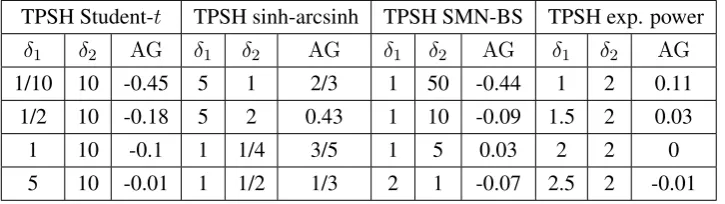
Figure 3:Asymmetry functionalCJfor: (a) TPSH Studentt; (b) TPSH exponential power; (c) TPSH SMN-BS; (d) TPSH sinh-arcsinh distribution. Lines correspond toδ1andδ2as in Table 1 and those values reversed.

2.3 Reparameterisations

For the TPSC family (4), Arellano-Valle et al. (2005) propose the reparameterisation(µ, σ1, σ2, δ) ↔

(µ, σ, γ, δ) using the transformation σ1 = σb(γ), σ2 = σa(γ), where {a(·), b(·)} are positive

TPSH Student-t TPSH sinh-arcsinh TPSH SMN-BS TPSH exp. power

δ1 δ2 AG δ1 δ2 AG δ1 δ2 AG δ1 δ2 AG

1/10 10 -0.45 5 1 2/3 1 50 -0.44 1 2 0.11 1/2 10 -0.18 5 2 0.43 1 10 -0.09 1.5 2 0.03 1 10 -0.1 1 1/4 3/5 1 5 0.03 2 2 0 5 10 -0.01 1 1/2 1/3 2 1 -0.07 2.5 2 -0.01

Table 1:Parameters used to obtain the functionals in Figure 3.

{a(γ), b(γ)_} = _{γ,1/γ_}, γ _∈ R+ (Fern´andez and Steel, 1998a), and the ϵ−skew parameterisation {a(γ), b(γ)_}=_{1₋γ,1 +γ_},γ _∈(₋1,1)(Mudholkar and Hutson, 2000). Jones and Anaya-Izquierdo (2010) and Rubio and Steel (2014) show that choosinga(γ) +b(γ)to be constant induces orthogonality betweenσ andγ. This reparameterisation is also appealing because the scalarγ can be interpreted as a skewness parameter since the AG measure of skewness depends only on this parameter. In particular, we obtain

AG = a(γ)−b(γ)

a(γ) +b(γ).

This reparameterisation can also be used in DTP distributions for inducing orthogonality between

σ andγ through parameterisations that verifya(γ) +b(γ) =constant. Under this reparameterisation, density (1) becomes

s(x;µ, σ, γ, δ1, δ2) = 2

σc(γ, δ1, δ2)

[

f(0;δ2)f

(

x₋µ

σb(γ);δ1

)

I(x < µ)+f(0;δ1)f

(

x₋µ

σa(γ);δ2

)

I(x_≥µ)

] ,

(8) wherec(γ, δ1, δ2) = b(γ)f(0;δ2) +a(γ)f(0;δ1). The interpretation ofγ in the wider DTP family is

slightly different since the cumulation of mass (and thus AG) depends also on the shape parameters

(δ1, δ2). However, the parameterγdoes not modify the shape ofs.

Using this reparameterisation we can obtain the “generalized asymmetric Student-t distribution” proposed in Zhu and Galbraith (2010) by taking f to be a Student-t density and _{a(γ), b(γ)_} =

{γ,1₋γ_}, γ _∈ (0,1). Under the same parameterisation, the “generalized asymmetric exponential power distribution” proposed in Zhu and Galbraith (2011) corresponds to an exponential power density forf.

For the TPSH family (5) there seems to be no obvious reparameterisation that induces parame-ter orthogonality. However, we can employ the reparameparame-terisationδ1 = δb∗(ζ), δ2 = δa∗(ζ), with {a∗(_·), b∗(_·)_}positive differentiable functions. This helps to separate the roles of the shape parameters, sinceδ can be interpreted as in the underlying symmetric model, whileζ explains the difference be-tween the shapes either side of the mode. The latter follows by noting thatδ1/δ2 =b∗(ζ)/a∗(ζ). This

reparameterisation can also be applied to the DTP family, leading to the following density

s(x;µ, σ, γ, δ, ζ) = 2

σc(γ, δ, ζ)

[

f(0;δa∗(ζ))f

(

x₋µ

σb(γ);δb

∗_(ζ)

)

I(x < µ)

+ f(0;δb∗(ζ))f (

x₋µ

σa(γ);δa

∗_(ζ)

)

I(x_≥µ)

]

wherec(γ, δ, ζ) =b(γ)f(0;δa∗_{(ζ)) +a(γ)f(0;δb}∗_(ζ)).

3

Bayesian Inference

3.1 Improper priors

In this section we propose a class of “benchmark” priors for the models studied in Section 2 with the parameterisations in (8) or (9). The proposed prior structure is inspired by the independence Jeffreys prior for the symmetric model, producing a scale and location-invariant prior.

The following result shows that the use of improper priors on the shape parameters of DTP models often leads to improper posteriors.

Theorem 1 Letx_{= (x1, ..., xn)be an independent sample from(8)and consider the prior structure}

p(µ, σ, γ, δ1, δ2)∝p(µ)p(σ)p(γ)p(δ1)p(δ2), (10)

wherep(δ1)and/orp(δ2)are improper priors. It follows that

(i) Iff(0;δ)does not depend uponδ, then the posterior is improper.

(ii) Iff(0;δ)is bounded from above, then a necessary condition for posterior propriety is

∫

∆

f(0;δi)np(δi)dδi<∞, i= 1,2. (11)

(iii) If f(0;δ) is a continuous and monotonic function of δ, then there exists M > 0 such that a necessary condition for the propriety of the posterior is

∫

∆

f(0;δi)n

[f(0;δi) +M]n

p(δi)dδi<∞, i= 1,2. (12)

This theorem provides a red flag for the use of improper priors on the shape parameters of DTP models. For instance, (i), (ii) and (iii) imply, respectively, that the use of improper priors on the shape pa-rameters(δ1, δ2)of DTP exponential power (with the parameterisation in Zhu and Zinde-Walsh, 2009),

DTP Student–t, and DTP sinh–arcsinh distributions leads to improper posteriors.

In DTP model (8) the parametersγ and(δ1, δ2)control the difference in the scale and the shapes

either side of the mode, respectively. So we adopt a product prior structurep(γ)p(δ1, δ2), allowing for

prior dependence betweenδ1 andδ2. The following result provides conditions for the existence of the

corresponding posterior distribution whenf is a scale mixture of normals. The case where the sample contains repeated observations is covered as well.

Theorem 2 Let x _{= (x1, ..., xn) be an independent sample from (8). Let f be a scale mixture of} normals and consider the prior structure

p(µ, σ, γ, δ1, δ2)∝

1

σp(γ)p(δ1, δ2), (13)

(i) The posterior distribution of(µ, σ, γ, δ1, δ2)is proper ifn≥2and all the observations are

differ-ent.

(ii) If x _{contains repeated observations, let k be the largest number of observations with the same}

value inx_{and1< k < n, then the posterior of(µ, σ, γ, δ1, δ2)is proper if and only if the mixing} distribution off satisfies fori= 1,2andjthe observation index

∫

0<τ1≤···≤τn<∞

τ_n−₋(n_k−2)/2 ∏

j̸=n−k,n

τ_j1/2dP(τ1,...,τn|δi)dδi<∞. (14)

In the case of a two-piece Student-tsampling model,(14)is equivalent to

∫ (k−1)/(n−k)+ξ

(k−1)/(n−k)

p(δi)

(n₋k)δi−(k−1)

dδi<∞ and

∫ (k−1)/(n−k)

0

p(δi)dδi = 0, (15)

for allξ >0andi= 1,2.

For the reparameterisation (9), the parameters(γ, δ, ζ)have separate roles:γcontrols the difference in the scale either side of the mode, δ represents the shape parameter of the underlying symmetric density, andζcontrols the difference in the shape either side of the mode. For this reason, it is reasonable to adopt an independent prior structure on these parameters. The following result provides conditions for the existence of the posterior distribution.

Remark 1 Letx_{= (x1, ..., xn)be an independent sample from(9). Letfbe a scale mixture of normals} and consider the prior structure

p(µ, σ, γ, δ, ζ)_∝ 1

σp(γ)p(δ)p(ζ), (16)

wherep(γ),p(δ), andp(ζ)are proper. The posterior distribution of(µ, σ, γ, δ, ζ)is proper ifn_≥2and all the observations are different. If the sample contains repeated observations, We need to check that the induced prior on(δ1, δ2), for the parameterisation (8), satisfies (14).

Proof.The results follows by a change of variable from(δ1, δ2)to(δ, ζ).

As discussed in previous sections, the parameters of a distribution obtained through the TPSC trans-formation,(µ, σ, γ, δ), can be interpreted as location, scale, skewness and shape, respectively. For this reason we adopt the product prior structurep(µ, σ, γ, δ) _∝ 1

σp(γ)p(δ)for this family. In TPSH

mod-els the shape parameters(δ1, δ2) control the mass cumulated on each side of the mode as well as the

shape. In addition, these parameters are not orthogonal in general. We therefore adopt the product prior

structurep(µ, σ, δ1, δ2) ∝

1

σp(δ1, δ2)in this family, wherep(δ1, δ2)denotes a proper joint distribution

which allows for prior dependence betweenδ1 andδ2. Theorem 2 covers the propriety of the posterior

under these priors for TPSC and TPSH sampling models. For TPSH models with the parameterisa-tion (9), Remark 1 provides condiparameterisa-tions for the existence of the posterior distribuparameterisa-tion under the prior

p(µ, σ, δ, ζ)_∝ 1

σp(δ)p(ζ).

0. In practice, this corresponds to any observation recorded with finite precision, as well as left, right and interval censoring. When the quantitative effect of censoring is not negligible, this must be formally taken into account. The following corollary provides conditions for the existence of the posterior from set observations with DTP sampling models.

Corollary 1 Let x _{= (S1, ..., Sn) be an independent sample of set observations from (8). Let f be} a scale mixture of normals and consider the prior structure (13). Then, the posterior distribution of

(µ, σ, γ, δ1, δ2)is proper ifn≥2and there exists a pair of sets, say(Si, Sj), such that

inf

xi∈Si,xj∈Sj|

xi−xj| > 0. (17)

Thus, whenever each sample of set observations contains at least two intervals that do not overlap, the posterior distribution of(µ, σ, γ, δ1, δ2)is proper. This result also applies to the parameterisation (9)

with prior (16).

3.2 Choice of the prior on(γ, δ, ζ)

We now propose specific priors for the parameters (γ, δ, ζ) in (16) for a general choice of f in (9), and its corresponding subfamilies. We employ the parameterisation_{a(γ), b(γ)_} = _{1₋γ,1 +γ_},

γ _∈(₋1,1)(so thatσ andγ are orthogonal), and_{a∗(ζ), b∗(ζ)_}= _{1₋ζ,1 +ζ_},ζ _∈ (₋1,1). The shape parameterδ typically controls the peakedness and the heaviness of tails of the density function. As mentioned earlier, the parametersγ andζ control the difference in scale and shape either side ofµ. This interpretability of the parameters facilitates the choice of hyperparameters. In particular, reasonable priors to reflect vague prior beliefs are thatγ _∼ Unif(₋1,1)andζ _∼ Unif(₋1,1). The elicitation of the prior on the parameterδ is more delicate, given that this parameter has different interpretations for different models. However, in all the models of interest,δ can be interpreted as a kurtosis parameter. Therefore, in order to come up with a more general elicitation strategy we propose basing this choice on a prior for a bounded kurtosis measure, which is common to all models and is an injective function of

δ, sayκ =κ(δ). The boundedness assumption onκallows us to assign a proper uniform prior on this quantity, while the injectivity is required for obtaining the induced prior on the parameterδby inverting this function. See Critchley and Jones (2008) for a good survey on kurtosis measures.

We propose to adopt the scalar kurtosis measure κ = 2 f(πR)

f(mode) −1 from Critchley and Jones

(2008), where πR represents the positive mode of −f′ (the inflection point). This measure κ takes

values in K _⊂ (₋1,1), assigning the value κ = 0.213 to the normal distribution. Numerically, we have found that κ is an injective function of δ for many distributions f, such as the Student-t, the symmetric sinh-arcsinh, the symmetric Johnson-SU, the exponential power withδ > 1, the symmetric

Algorithm 1Construction of the prior onδ.

1: Identify the rangeKcovered by varyingδin the model of interest.

2: Simulateu_{= (u1, . . . , uN)∼Unif(K).}

3: Calculated_=κ−1₍u_).

4: Approximate the distribution ofd_{using a kernel density estimator.}

0 5 10 15 20

0.0

0.1

0.2

0.3

0.4

δ 0 1 2 3 4 5

0.0

0.5

1.0

1.5

δ

(a) (b)

Figure 4:Priors forδ: (a) Student-tdistribution; (b) Sinh-arcsinh distribution.

3.3 Weakly informative priors

We may prefer to use a “vague” proper prior which is not very influential on the posterior inference. In the previous section we provided weakly informative priors for the shape parameters(γ, δ, ζ). We can combine that with independent vague proper priors on the location and scale parameters(µ, σ). For the location parameter we propose a uniform prior on an appropriate bounded interval_D, while for the scale parameter we employ a Half-Cauchy distribution with location0and scales(Polson and Scott, 2012). Unfortunately, general choices for_Dandsare not available, given that these values depend on the units of measurement. We recommend conducting sensitivity analyses with respect to_Dands. Note that the structure of this prior resembles that of the improper benchmark priors discussed in the previous sections.

This prior structure is also useful for choices offthat do not belong to the family of scale mixtures of normals and, consequently, the existence of the posterior under improper priors is not covered by the results in Subsection 3.1.

4

Applications

We present three examples with real data to illustrate the use of DTP, TPSC and TPSH distributions. We adopt theϵ₋skew parameterisation for DTP and TPSC models. In the first two examples, simulations of the posterior distributions are obtained using thet-walk algorithm (Christen and Fox, 2010). Given the hierarchical nature of the third example, we use the adaptive Metropolis within Gibbs sampler imple-mented in the R package ‘spBayes’ (Finley and Banerjee, 2013). R codes used here and the R-package ‘DTP’, which implements basic functions related to the proposed models, are available on request.

non-nested choices forf. We also compare the DTP model and its submodels with other distributions used in the literature. For a fair model comparison, we include appropriate competitors in each example, matched to the features of the data. A meaningful Bayesian comparison with these other models would require the specification of priors for the parameters in these other distributions that are comparable (matched) to our models, and to compute Bayes factors we would need to use proper priors for all model-specific parameters. This would be a nontrivial undertaking and would risk diluting the main message of the paper. We choose instead to compare with these other classes of distributions through classical information criteria based on maximum likelihood estimates (MLE). We aim to show that our DTP families are flexible enough and then we can use formal Bayesian methods to select (or average) models within these families.

Given that DTP, TPSC, and TPSH distributions capture different sorts of asymmetry, conducting model comparison between these distributions not only provides information about which model fits the data better but it also indicates what kind of asymmetry is favoured by the data. In addition, the DTP family provides important advantages in terms of interpretability of parameters (and, thus, prior elicitation) and inferential properties.

4.1 Internet traffic data

In this example we analyse the teletraffic data set studied in Ramirez-Cobo et al. (2010), which contains

n = 3143observations, representing transferred bytes/sec within consecutive seconds. Ramirez-Cobo et al. (2010) propose the use of a Normal Laplace distribution to model these data after a logarithmic transformation. The Normal Laplace distribution is obtained as the convolution of a Normal distribution and a two–piece Laplace distribution with location0and two parameters(α, β)that jointly control the scale and the skewness. The Normal Laplace distribution has tails heavier than those of the normal distribution (Reed and Jorgensen, 2004). We also use the sinh-arcsinh distribution of Jones and Pewsey (2009), indicated by sJP and the skew-tof Azzalini and Capitanio (2003), denoted by sAC (see

Ap-pendix A). Here, we explore the performance of the DTP sinh–arcsinh distribution (DTP SAS). This distribution allows for all moments to exist and accommodates both heavier and lighter tails than the normal distribution, which is a submodel of the DTP SAS (δ1 = δ2 = 1,γ = 0). We use the priors

of Subsection 3.3: µ_∼Unif(0,25), σ _∼HalfCauchy(0, s), γ _∼Unif(₋1,1), ζ _∼ Unif(₋1,1),where

Model µ_{b b}σ _bγ bδ ζb AIC BIC DTP SAS 11.16 11.39 -0.98 10.795 -0.94 5849.14 5879.40

TPSC SAS 11.80 0.85 0.14 1.26 – 5884.95 5909.16 TPSH SAS 11.75 0.87 – 1.30 -0.08 5880.20 5904.41

sJP 11.78 0.84 (εb) -0.16 1.25 – 5886.84 5911.05

Normal Laplace 11.77 8.39 (α_b) 4.09 (βb) 0.56 – 5922.73 5946.94

sAC 12.07 0.75 (bλ) -0.98 1057.40 – 5919.52 5943.73

Table 2:Internet traffic data: Maximum likelihood estimates, AIC and BIC (best values in bold).

8 9 10 11 12 13 14

0.0

0.1

0.2

0.3

0.4

0.5

0.6

0.7

8 9 10 11 12 13 14

−15

−10

−5

0

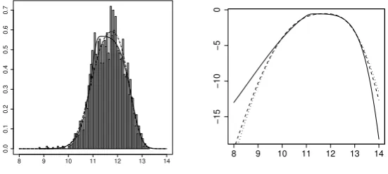
Figure 5: Internet traffic data (in logarithms; histogram) with (a) Predictive densities and (b) Log-predictive densities: DTP (continuous line); TPSH (dashed line); TPSC (dotted line).

Model DTP SAS TPSH SAS TPSC SAS TPSC normal Symm. SAS normal

BF 1 _≈0 _≈0 _≈0 _≈0 _≈0

Table 3:Internet traffic data. Bayes factors of submodels vs. DTP SAS model (entries<10−100_).

4.2 Actuarial Application

In this application we analyse the claim sizes reported in Berlaint et al. (2004) which can be found in

http://lstat.kuleuven.be/Wiley/. This data set containsn= 1823observations provided by the reinsurance brokers Aon Re Belgium. Such data typically contain extreme observations, and the logarithmic transformation is often used to reduce the effect of these extreme values (Ramirez-Cobo et al., 2010). A quantity of interest in this context is the probability that the claims exceed a certain bound (Venturini et al., 2008). This is often used for budgetary planning, which emphasises the importance of properly modelling the tails of the distribution.

for the Student-tmodel we truncateδ >2and restrictζ _∈(₋0.99,0.99). This truncation guarantees that condition (15) is satisfied since it implies thatδ1, δ2>(k−1)/(n−k)≈0.02. For the SMN-BS model,

theκmeasure is injective only on the intervalδ _∈(0,2.65), which covers the rangeκ_∈(0.213,0.560). In addition, for this model we can check that condition (14) is satisfied if we truncate theδi’s away from

zero,e.g.by imposingδ >1_×10−6 and takingζ _∈(₋0.999,0.999). Thus, we restrict the prior forδ

in the SMN-BS model to(1_×10−6,2.65). The posterior distributions are proper by Remark 1.

We also use the skew-tdistributions in Azzalini and Capitanio (2003) (sAC) and Jones and Faddy

(2003), denoted bysJF (see Appendix A). Table 4 shows the MLE and the AIC and BIC criteria, which

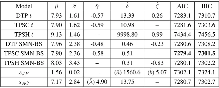
favour the TPSC SMN-BS model overall. The Bayes factors, reported in Table 5, favour the TPSC model for both underlying choices off and favours the TPSC SMN-BS model overall, which agrees with the conclusion from AIC and BIC. However, there is no conclusive message from the SMN-BS models about which type of asymmetry is best for the data. The TSPH variant does almost as well. This is in line with the fact that the SMN-BS model does not distinguish clearly between TPSH and TPSC transformations, as discussed in Subsection 2.2. In contrast, the Student-tmodels, for which both transformations are very distinct, unambiguously indicate that the asymmetry is in the main body of the data and not in the tails: the TPSHtmodel does very badly indeed, using both classical and Bayesian methods. Figure 6 shows the corresponding predictive densities and illustrates the poor fit of the TPSHt

model which clearly affects the estimation of the right-tail probabilities shown in Figure 6(b): this model produces a predictive probability of 0.01 for the eventx >17, while the other models lead to a predictive probability of less than 0.004. Unlike in the previous application, where right “main-body” skewness is combined with a heavier left tail (bothγ andζ are estimated to be highly negative), the skew-t by Azzalini and Capitanio (2003) does well here, as these data combine right skewness in the main body with a fatter right tail. This is a feature that thesAC imposes (for positiveλwith both asymmetries in

the opposite direction forλ <0). It is important to point out that the DTP families are not restricted in this way, as evidenced by the superiority of the DTP model in the previous application.

Model µˆ σˆ γˆ δˆ ζˆ AIC BIC

DTPt 7.93 1.61 -0.57 13.33 0.26 7283.1 7310.7 TPSCt 7.90 1.62 -0.59 10.98 – 7281.6 7303.6 TPSHt 9.13 1.46 – 9998.80 0.99 7434.4 7456.5 DTP SMN-BS 7.96 2.38 -0.48 0.46 -0.23 7280.6 7308.2 TPSC SMN-BS 7.90 2.36 -0.58 0.51 – 7279.4 7301.5

TPSH SMN-BS 8.03 3.43 – 0.31 -0.83 7280.1 7302.2

sJF 1.56 0.02 – (ˆa) 1560.6 (ˆb) 5.07 7302.1 7324.1 sAC 7.17 2.84 (ˆλ) 4.90 13.75 – 7280.7 7302.7

Model DTP TPSH TPSC Student-t 1 5.00_×10−65 _2.05

SMN-BS 4.50 1.61 9.02

Table 5:Aon data: Bayes factors with respect to the DTP-tmodel.

4.3 Hierarchical Bayesian Models in Meta–Analysis

Bayesian hierarchical models are used in a variety of applied contexts to tackle parameter heterogeneity. A common example of this is the two–level normal model:

yj|θj ∼ N(θj, σj), j= 1. . . n,

θj ∼ N(µ, σ). (18)

A natural question is whether the assumption of normality of the random effects is appropriate: the implications of departures from this assumption are discussed in Zhang and Davidian (2001), Thompson and Lee (2008) and McCulloch and Neuhaus (2011).

In order to produce models that are robust to departures from normality ofθj, several generalisations

of (18) have been proposed. For example, Doss and Hobert (2010) employ a Student–t distribution, Thompson and Lee (2008) use a TPSC t distribution withδ > 2 degrees of freedom, while Dunson (2010) follows a Bayesian nonparametric approach. The use of non–normal distributional assumptions in this hierarchical model typically requires more sophisticated MCMC methods as discussed in Roberts and Rosental (2009).

4.3.1 Fluoride Meta–analysis

In this example we analyse the data set presented in Marinho et al. (2003) and used in Thompson and Lee (2008), which containsn= 70trials assessing the effectiveness of fluoride toothpaste compared to a placebo conducted between 1954 and 1994. The treatment effect is the “prevented fraction”, defined as the mean increment in the controls minus the mean increment in the treated group, divided by the mean increment in the controls. Thompson and Lee (2008) then propose the model

yj|θj ∼ N(θj, σj),

θj ∼ P, (19)

where yj is the estimate of the treatment effect in study j, θj is the true treatment effect in studyj,

and the parametersσj are estimated from the data and assumed known. They compare the conclusions

obtained for the true treatment effect for the following choices for P: (i) a TPSC tdistribution with

δ >2degrees of freedom, (ii) a symmetric Studenttdistribution withδ >2degrees of freedom, (iii) a

TPSC normal distribution, and (iv) a normal distribution.

Here, we study six choices forP: (i) a normal distribution, (ii) a symmetric sinh–arcsinh (SAS) distribution, (iii) a TPSC normal distribution, (iv) a TPSC SAS distribution, (v) a TPSH SAS distribution and (vi) a DTP SAS distribution. For the DTP model, we adopt the prior structure as in Subsection

5 10 15 20

0.00

0.05

0.10

0.15

0.20

0.25

0.30

5 10 15 20

−10

−8

−6

−4

−2

(a) (b)

5 10 15 20

0.00

0.05

0.10

0.15

0.20

0.25

0.30

5 10 15 20

−10

−8

−6

−4

−2

(c) (d)

Figure 6: Aon data (histogram) with (a) Predictive densities and (b) Log-predictive densities: DTPt(continuous line); TPSHt(dashed line); TPSCt(dotted line). (c) Predictive densities and (d) Log-predictive densities: DTP SMN-BS (continuous line); TPSH SMN-BS (dashed line); TPSC SMN-BS (dotted line).

Unif(₋1,1), δ_∼p(δ), ζ _∼Unif(₋1,1), with the prior shown in Figure 4 forδ, ands= 1/5,1,5. The results were not sensitive to the choice ofs.

Figure 7 shows the posterior predictive densities for the treatment effect under different distribu-tional assumptions for the random effects. Clearly, symmetric distributions put more predictive mass in the left tail(_−∞,0.05)than those with asymmetry. Therefore, the probability of a small or a negative effect is overestimated under symmetric random effects. The predictive distributions obtained for DTP, TPSC, and TPSH SAS models are fairly similar in this case. However, the Bayes factors, shown in Table 6, favour DTP and TPSH SAS models over the other competitors.

Model DTP SAS TPSH SAS TPSC SAS TPSC normal Sym. SAS normal

BF 1 1.27 0.30 0.05 0.02 5.2_×10−5

−0.2 0.0 0.2 0.4 0.6

0

2

4

6

−0.2 0.0 0.2 0.4 0.6

0

2

4

6

−0.2 0.0 0.2 0.4 0.6

0

2

4

6

(a) (b) (c)

−0.2 0.0 0.2 0.4 0.6

0

2

4

6

−0.2 0.0 0.2 0.4 0.6

0

2

4

6

−0.2 0.0 0.2 0.4 0.6

0

2

4

6

(d) (e) (f)

Figure 7: Predictive densities for the treatment effect: (a) Normal; (b) Symmetric SAS; (c) TPSC normal; (d) TPSC SAS; (e) TPSH SAS; (f) DTP SAS.

5

Concluding Remarks

We introduce a simple, intuitive and general class of transformations (DTP) that produces flexible uni-modal and continuous distributions with parameters that separately control main-body skewness and tails on each side of the mode. Although some particular cases of DTP models have already appeared (Zhu and Galbraith, 2010, 2011), we formalise the idea and extend it to a wide range of symmetric “base” distributions_F. We also distinguish two subclasses of transformations and examine their inter-pretation as skewing mechanisms. A considerable advantage of the DTP class of transformations is the interpretability of its parameters (see Jones, 2014 for the importance of interpretability) which, in the Bayesian context, also facilitates prior elicitation. We propose a scale and location-invariant prior struc-ture and derive conditions for posterior existence, also taking into account repeated and set observations.

As illustrated by the applications, DTP families provide a flexible way of modelling unimodal data (or latent effects with unimodal distributions) and we provide a Bayesian framework for inference with sensible prior assumptions. In addition, we can conduct formal model comparison through Bayes factors for selecting models within the following classes:

• subclasses of DTP models with the same underlying symmetric base distributionf: this is possible through the clearly separated roles of the parameters and the ensuing product prior structure with proper priors onγ andζ.

on the kurtosis measureκ.

DTP, TPSC and TPSH transformations can be used to construct robust models and, since they capture different kinds of asymmetry, selecting between these models provides more insight into the features of a data set. We have used Bayes factors for model choice, but other criteria, such as log-predictive scores, might be considered as well.

DTP families can be extended to the multivariate case in several ways. For TPSC models, Ferreira and Steel (2007) propose the use of affine transformations to produce a multivariate extension while Rubio and Steel (2013) propose to use copulas. In a similar fashion, the DTP (and consequently the TPSH) family can be used to construct multivariate distributions.

A different subclass of DTP transformations can be obtained by fixingσ1=σandσ2 =

f(0;δ2)

f(0;δ1)

σ,

leading to distributions with different shapes but equal mass cumulated on each side of the mode. This idea is proposed in Rubio (2013), who also composes this transformation with other skewing mecha-nisms to produce a different type of generalised skew-tdistribution.

Rubio and Steel (2014) explore the use of Jeffreys priors in TPSC models. The use of Jeffreys priors for TPSH and DTP models is the object of further research.

Appendix A: Some density functions

(i) The symmetric Johnson-SUdistribution (Johnson, 1949):

f(x;µ, σ, δ) = δ

σϕ

[

δarcsinh

(

x₋µ

σ

)] (

1 +

(

x₋µ

σ

)2)−12 .

(ii) The sinh-arcsinh distribution (Jones and Pewsey, 2009):

sJP(x;µ, σ, δ) =

δ σϕ [ sinh ( δarcsinh (

x₋µ

σ ) −ε )]cosh ( δarcsinh (

x₋µ

σ ) −ε ) √ 1 + (

x₋µ

σ

)2 ,

whereε_∈Rcontrols the asymmetry of the density and symmetry corresponds toε= 0. (iii) SMN-BS, a scale mixture of normals with Birnbaum-Saunders(δ, δ)mixing:

f(x;µ, σ, δ) =

eδ12

(_√

δx2_{+ 1K}

0

(√

δx2₊₁

δ2

)

+K1

(√

δx2₊₁

δ2

))

2πδ3/2√_δx2_{+ 1} .

whereKn(z)represents the modified Bessel function of the second kind.

(iv) The skew-tdensity from Jones and Faddy (2003):

sJF(x;µ, σ, a, b) =C_a,b−1

[

1 +_√ t

a+b+t2

]a+1/2[

1_−√ t

a+b+t2

]b+1/2 ,

wherea, b >0,Ca,b = 2a+b−1Beta(a, b)√a+b, andt =

x₋µ

σ . The parameters(a, b)control

the tails and skewness jointly. The density sJF is asymmetric if and only if a ̸= b, so that the

(v) The skew-tdensity from Azzalini and Capitanio (2003):

sAC(x;µ, σ, λ, δ) = 2f(x;µ, σ, δ)F

( λx

√

δ+ 1

δ+x2;µ, σ, δ+ 1

) ,

whereλ _∈Randf andF are, respectively, the density function and the distribution function of the Student-t.

Appendix B: Proofs

Proof of Theorem 1

The marginal likelihood of the data can be bounded from below as follows

m(x_{) ∝}

∫ ∆ ∫ ∆ ∫ Γ ∫ R+ ∫ R   n ∏ j=1

s(xj;µ, σ, γ, δ1, δ2)



p(µ)p(σ)p(γ)p(δ1)p(δ2)dµdσdγdδ1dδ2

≥ ∫ ∆ ∫ ∆ ∫ Γ ∫ R+ ∫ x(1)

−∞

f(0;δ1)n

σn_H(γ)n_[f(0;δ

1) +f(0;δ2)]n   n ∏ j=1 f (

xj−µ

σa(γ);δ2

)



× p(µ)p(σ)p(γ)p(δ1)p(δ2)dµdσdγdδ1dδ2 (20)

wheres(_·)is given by (8) in the paper,H(γ) = max_{a(γ), b(γ)_}, andx(1)represents the smallest order

statistic ofx_{. Therefore:}

(i) follows by noting that the lower bound (20) does not depend uponδ1.

(ii) follows by using the following inequality, providedf(0;δ)_≤U for someU >0

f(0;δ1)n

[f(0;δ1) +f(0;δ2)]n ≥

f(0;δ1)n

2n_Un ,

which leads to the necessary condition (11).

(iii) Given thatf(0;δ) is continuous and monotonic, there existM > 0and a set∆2(M) ⊂∆such

thatf(0;δ) < M for allδ _∈ ∆2(M). If we integrateδ2 over∆2, we obtain the following lower

bound, up to a proportionality constant, form(x₎

∫ ∆2 ∫ ∆ ∫ Γ ∫ R+ ∫ x(1)

−∞

f(0;δ1)n

σn_H(γ)n_[f(0;δ

1) +f(0;δ2)]n   n ∏ j=1 f (

xj−µ

σa(γ);δ2

)



× p(µ)p(σ)p(γ)p(δ1)p(δ2)dµdσdγdδ1dδ2

≥ ∫ ∆2 ∫ ∆ ∫ Γ ∫ R+ ∫ x(1)

−∞

f(0;δ1)n

σn_H(γ)n_[f(0;δ

1) +M]n   n ∏ j=1 f (

xj −µ

σa(γ);δ2

)



× p(µ)p(σ)p(γ)p(δ1)p(δ2)dµdσdγdδ1dδ2.

Analogous results can be obtained forδ2by integratingµover(x(n),∞), wherex(n)represents the

largest order statistic ofx_.

Proof of Theorem 2

(i) In this parameterization,εin (2) does not depend onσ. This fact will be used implicitly in a change of variable below. We obtain

p(x_{) ∝}

∫ ∆ ∫ ∆ ∫ _∞ 0 ∫ _∞ −∞ ∫ Rn + 1 [a(γ) +b(γ)]n

∏n

j=1λ

1 2 j

σn+1 exp



₋ 1

2σ2 n ∑

j=1

λj

ij(γ)2

(xj−µ)2  

× p(γδ1, δ2)

n ∏

j=1 {

εdP_λj|δ1I(xj < µ) + (1−ε)dPλj|δ2I(xj ≥µ)

}

dµdσdγdδ1dδ2

≤ ∫ ∆ ∫ ∆ ∫ _∞ 0 ∫ _∞ −∞ ∫ Rn + 1 [a(γ) +b(γ)]n

∏n

j=1λ

1 2 j

σn+1 exp



₋ 1

2σ2_h(γ)2 n ∑

j=1

λj(xj −µ)2

 

× p(γ)p(δ1, δ2)

n ∏

j=1 {

εdPλj|δ1I(xj < µ) + (1−ε)dPλj|δ2I(xj ≥µ)

}

dµdσdγdδ1dδ2,

whereij(γ) =a(γ)I(xj ≥µ) +b(γ)I(xj < µ)andh(γ) = max{a(γ), b(γ)}. Now, consider the

change of variableθ=σh(γ), then we get that this upper bound can be written as follows

∫ ∆ ∫ ∆ ∫ _∞ 0 ∫ _∞ −∞ ∫ Rn +

h(γ)n

[a(γ) +b(γ)]n ∏n

j=1λ

1 2 j

θn+1 exp



₋ 1

2θ2 n ∑

j=1

λj(xj−µ)2

 

× p(γ)p(δ1, δ2)

n ∏

j=1 {

εdP_λj|δ1I(xj < µ) + (1−ε)dPλj|δ2I(xj ≥µ)

}

dµdθdγdδ1dδ2.

By using that0_≤ε_≤1, 1

2 ≤

h(γ)n

[a(γ) +b(γ)]n ≤1it follows that the propriety of the posterior of

(µ, σ, γ, δ1, δ2)under this prior structure is equivalent to the propriety of the posterior distribution

of a TPSH sampling model with parameters (µ, σ, δ1, δ1) and prior structure π(µ, σ, δ1, δ1) ∝ σ−1p(δ1, δ2), where p(δ1, δ2) is a proper prior. The rest of the proof thus focuses on the latter

model, for which, by construction, we have

f(xj;µ, σ, δ1, δ2) =

∫ _∞ 0 2λ 1 2 j √

2πσ exp [

−₂λ_σj₂(xj −µ)2

]

× {εdPλj|δ1I(xj < µ) + (1−ε)dPλj|δ2I(xj ≥µ)

} ,

withεas in (2). Then, we can write the marginal ofx_{as follows}

p(x_{) ∝}

∫ ∆ ∫ ∆ ∫ _∞ 0 ∫ _∞ −∞ ∫ Rn + ∏n j=1λ 1 2 j

σn+1 exp



₋ 1

2σ2 n ∑

j=1

λj(xj−µ)2



p(δ1, δ2)

× n ∏

j=1 {

εdP_λj|δ1I(xj < µ) + (1−ε)dPλj|δ2I(xj ≥µ)

}

Separating the integral with respect toµinton+1integrals over the domains(_−∞, x₍₁₎),[x₍₁₎, x₍₂₎), ...,[x(n),∞), we have that

I1 =

∫ ∆ ∫ ∆ ∫ _∞ 0

∫ x(1)

−∞ ∫ Rn + ∏n j=1λ 1 2 j

σn+1 exp



₋ 1

2σ2 n ∑

j=1

λj(xj−µ)2

 

× p(δ1, δ2)(1−ε)n

n ∏

j=1

dP_λj|δ2dµdσdδ1dδ2.

By noting that 0 _≤ ε _≤ 1, extending the integration domain on µ to the whole real line and integrating outδ1 we obtain

I1≤

∫ ∆ ∫ _∞ 0 ∫ _∞ −∞ ∫

Rn+ ∏n

j=1λ

1 2 j

σn+1 exp



₋ 1

2σ2 n ∑

j=1

λj(xj −µ)2

 p(δ2)

n ∏

j=1

dPλj|δ2dµdσdδ2<∞.

The finiteness of this integral is obtained using Theorem 1 from Fern´andez and Steel (1998b). Now, using similar arguments we have that

I2 =

∫ ∆ ∫ ∆ ∫ _∞ 0 ∫ _∞

x(n)

∫ Rn + ∏n j=1λ 1 2 j

σn+1 exp



₋ 1

2σ2 n ∑

j=1

λj(xj−µ)2

 

× p(δ1, δ2)εn

n ∏

j=1

dPλj|δ1dµdσdδ1dδ2

≤ ∫ ∆ ∫ ∞ 0 ∫ ∞ −∞ ∫

Rn+ ∏n

j=1λ

1 2 j

σn+1 exp



₋ 1

2σ2 n ∑

j=1

λj(xj−µ)2

 

× p(δ1)

n ∏

j=1

dP_λj|δ1dµdσdδ1 <∞.

Finally, for an intermediate region we have

I3 =

∫ ∆ ∫ ∆ ∫ _∞ 0

∫ x(k+1)

x(k)

∫ Rn + ∏n j=1λ 1 2 j

σn+1 exp



₋ 1

2σ2 n ∑

j=1

λj(x(j)−µ)2



p(δ1, δ2)εk(1−ε)n−k

× k ∏

j=1

dPλj|δ1

n ∏

j=k+1

dPλj|δ2dµdσdδ1dδ2

≤ ∫ ∆ ∫ ∆ ∫ _∞ 0 ∫ _∞ −∞ ∫ Rn + ∏n j=1λ 1 2 j

σn+1 exp



₋ 1

2σ2 n ∑

j=1

λj(x(j)−µ)2



p(δ1, δ2)

× k ∏

j=1

dP_λj|δ1

n ∏

j=k+1

dP_λj|δ2dµdσdδ1dδ2<∞.

The finiteness follows again from Theorem 1 from Fern´andez and Steel (1998b). Combining the finiteness ofI1,I2andI3the result follows.

Proof of Corollary 1

From the proof of point (i) in Theorem 1 it follows that the propriety of the posterior distribution

of (µ, σ, γ, δ1, δ2) is equivalent to proving the propriety of (µ, σ, δ), assuming that S1, . . . , Sn is an

i.i.d. sample of set observations from a scale mixture of normals f(_·;µ, σ, δ) and adopting the prior

π(µ, σ, δ)_∝σ−1_{p(δ), wherep(δ)is proper. The result then follows by combining this fact with}

Theo-rem 4 from Fern´andez and Steel (1998b).

References

Aas, K., and Haff, I. H. (2006), “The Generalized Hyperbolic Skew Student’st₋distribution,” Journal of Financial Econometrics, 4, 275–309.

Arnold, B. C., and Groeneveld, R. A. (1995), “Measuring Skewness With Respect to the Mode,”The American Statistician, 49, 34–38.

Arellano-Valle, R. B., G´omez, H. W., and Quintana, F. A. (2005), “Statistical Inference for a General Class of Asymmetric Distributions,”Journal of Statistical Planning and Inference, 128, 427–443.

Azzalini, A. (1985), “A Class of Distributions Which Includes the Normal Ones,”Scandinavian Journal of Statistics, 12, 171-178.

Azzalini, A. (1986), “Further Results on a Class of Distributions Which Includes the Normal Ones,” Statistica, 46, 199–208.

Azzalini, A., and Capitanio, A. (2003), “Distributions Generated by Perturbation of Symmetry With Emphasis on a Multivariate Skew-t Distribution,”Journal of the Royal Statistical Society B, 65, 367– 389.

Barndorff-Nielsen, O. E. (1977), “Exponentially Decreasing Distributions for the Logarithm of Particle Size,”Proceedings of the Royal Society of London A, 353, 401-419.

Berlaint, J., Goegebeur, Y., Segers, J., and Teugels, J. (2004),Statistics of Extremes: Theory and Appli-cations, Wiley, New York.

Christen, J. A., and Fox, C. (2010), “A General Purpose Sampling Algorithm for Continuous Distribu-tions (The t-walk),”Bayesian Analysis, 5, 1–20.

Critchley, F., and Jones, M. C. (2008), “Asymmetry and Gradient Asymmetry Functions: Density-Based Skewness and Kurtosis,”Scandinavian Journal of Statistics, 35, 415-437.

Doss, H., and Hobert, J. P. (2010), “Estimation of Bayes Factors in a Class of Hierarchical Random Ef-fects Models Using Geometrically Ergodic MCMC Algorithm,”Journal of Computational and Graph-ical Statistics, 19, 295–312.

Fern´andez, C., Osiewalski, J., and Steel, M. F. J. (1995), “Modeling and Inference With v-Spherical Distributions,”Journal of the American Statistical Association, 90, 1331-1340.

Fern´andez, C., and Steel, M. F. J. (1998a), “On Bayesian Modeling of Fat Tails and Skewness,”Journal of the American Statistical Association, 93, 359–371.

Fern´andez, C. and Steel, M. F. J. (1998b). On the dangers of modelling through continuous distributions: A Bayesian perspective, in Bernardo, J. M., Berger, J. O., Dawid, A. P. and Smith, A. F. M. eds., Bayesian Statistics 6, Oxford University Press (with discussion), pp. 213–238.

Fern´andez, C., and Steel, M. F. J. (2000), “Bayesian Regression Analysis With Scale Mixtures of Nor-mals,”Econometric Theory, 16, 80–101.

Ferreira, J. T. A. S., and Steel, M. F. J. (2006), “A Constructive Representation of Univariate Skewed Distributions,”Journal of the American Statistical Association, 101, 823–829.

Ferreira, J. T. A. S., and Steel, M. F. J. (2007), “A New Class of Skewed Multivariate Distributions With Applications to Regression Analysis,”Statistica Sinica, 17, 505–529.

Finley, A. O., and Banerjee, S. (2013), “spBayes: Univariate and Multivariate Spatial-temporal Model-ing,” R package version 0.3-8,http://CRAN.R-project.org/package=spBayes.

Fischer, M., and Klein, I. (2004), “Kurtosis Modelling by Means of the J₋Transformation,” Allge-meines Statistisches Archiv, 88, 35–50.

Goerg, G. M. (2011), “Lambert W Random Variables - A New Generalized Family of Skewed Distribu-tions with ApplicaDistribu-tions to Risk Estimation,”The Annals of Applied Statistics, 5, 2197–2230.

Groeneveld, R. A., and Meeden, G. (1984), “Measuring Skewness and Kurtosis,”The Statistician, 33, 391-399.

Hansen, B. E. (1994), “Autoregressive Conditional Density Estimation,” International Economic Re-view, 35, 705–730.

Haynes, M. A., MacGilllivray, H. L., and Mergersen, K. L. (1997), “Robustness of Ranking and Selec-tion Rules Using Generalized g and k DistribuSelec-tions,” Journal of Statistical Planning and Inference, 65, 45–66.

Johnson, N. L. (1949), “Systems of Frequency Curves Generated by Methods of Translation,” Biometrika, 36, 149–176.

Jones, M. C. (2014), “On Families of Distributions With Shape Parameters,” International Statistical Review, in press (with discussion).

Jones, M. C., and Anaya-Izquierdo K. (2010), “On Parameter Orthogonality in Symmetric and Skew Models,”Journal of Statistical Planning and Inference, 141, 758–770.

Jones, M. C., and Faddy, M. J. (2003), “A Skew Extension of the t-Distribution, With Applications,” Journal of Royal Statistical Society Series B, 65, 159–174.

Klein, I., and Fischer, M. (2006), “Power Kurtosis Transformations: Definition, Properties and Order-ing,”Allgemeines Statistisches Archiv, 90, 395–401.

Ley, C., and Paindaveine, D. (2010), “Multivariate Skewing Mechanisms: A Unified Perspective Based On the Transformation Approach,”Statistics&Probability Letters, 80, 1685–1694.

Marinho, V. C. C., Higgins, J. P. T., Logan, S., and Sheiham, A. (2003), “Fluoride Toothpastes for Preventing Dental Caries in Children and Adolescents (Cochrane Review),”The Cochrane Library, (Issue 4 edn). Wiley: Chichester.

McCulloch, M. E., and Neuhaus, J. M. (2011), “Misspecifying the Shape of a Random Effects Distribu-tion: Why Getting It Wrong May Not Matter,”Statistical Science, 26, 388–402.

Mudholkar, G. S., and Hutson, A. D. (2000), “The Epsilon-skew-normal Distribution for Analyzing Near-normal Data”Journal of Statistical Planning and Inference, 83, 291–309.

Polson, N., and Scott, J. G. (2012), “On the Half-Cauchy Prior for a Global Scale Parameter,”Bayesian Analysis, 7, 887–902.

Ramirez-Cobo, P., Lillo, R. E., Wilson, S., and Wiper, M. P. (2010), “Bayesian Inference for Double Pareto Lognormal Queues,”The Annals of Applied Statistics, 4, 1533–1557.

Reed, W., and Jorgensen, M. (2004), “The double Pareto-lognormal Distribution – A New Parametric Model for Size Distributions,”Communications in Statistics, Theory & Methods, 33, 1733-1753.

Roberts, G. O., and Rosenthal, J. S. (2009), “Examples of Adaptive MCMC,”Journal of Computational and Graphical Statistics, 18, 349–367.

Rosco, J. F., Jones, M. C., and Pewsey, A. (2011), “SkewtDistributions Via the Sinh-arcsinh Transfor-mation,”TEST 20: 630–652.

Rubio, F. J. (2013),Modelling of Kurtosis and Skewness: Bayesian Inference and Distribution Theory, PhD Thesis, University of Warwick, UK.

Rubio, F. J., and Steel, M. F. J. (2013), “Bayesian Inference for P(X < Y)Using Asymmetric Depen-dent Distributions,”Bayesian Analyisis, 8, 43–62.

Rubio, F. J., and Steel, M. F. J. (2014), “Inference in Two-Piece Location-Scale models With Jeffreys Priors (with discussion),”Bayesian Analyisis, 9, 1–22.

Thompson, S. G., and Lee, K. J. (2008), “Flexible Parametric Models for Random–Effects Distribu-tions,”Statistics in Medicine, 27, 418–434.

Tukey, J. M. (1977),Exploratory Data Analysis, Addison-Wesley, Reading, M. A.

van Zwet, W. R. (1964),Convex Transformations of Random Variables, Mathematisch Centrum, Ams-terdam.

Wang, J., Boyer, J., and Genton M. C. (2004), “A Skew Symmetric Representation of Multivariate Distributions,”Statistica Sinica, 14, 1259–1270.

Zhang, D., and Davidian, M. (2001). “Linear Mixed Models with Flexible Distributions of Random Effects for Longitudinal Data,”Biometrics 57, 795–802.

Zhu, D., and Galbraith, J. W. (2010), “A Generalized Asymmetric Student-t Distribution With Applica-tion to Financial Econometrics,”Journal of Econometrics, 157, 297–305.

Zhu, D., and Galbraith, J. W. (2011), “Modeling and Forecasting Expected Shortfall With the General-ized Asymmetric Student-tand Asymmetric Exponential Power Distributions,”Journal of Empirical Finance, 18, 765–778.