Optimal Portfolio Strategy with Discounted Stochastic
Cash Inflows
Charles I. Nkeki
Department of Mathematics, Faculty of Physical Sciences, University of Benin, Benin City, Nigeria
Email: nkekicharles2003@yahoo.com
Received March 19, 2012; revised June 10, 2012; accepted June 25, 2012
ABSTRACT
This paper examines optimal portfolios with discounted stochastic cash inflows (SCI). The cash inflows are invested into a market that is characterized by inflation-linked bond, a stock and a cash account. It was assumed that inflation- linked bond, stock and the cash inflows are stochastic and follow a standard geometric Brownian motion. The vari- ational form of Merton portfolio strategy was obtained by assuming that the investor chooses constant relative risk averse (CRRA) utility function. The inter-temporal hedging terms that offset any shock to the SCI were obtained. A closed form solution to our resulting non-linear partial differential equation was obtained.
Keywords: Optimal Portfolio; Stochastic Cash Inflows; Inflation-Linked Bond; Variational Form; Intertemporal Hedging Terms
1. Introduction
This paper consider the optimal portfolio strategies with valuing expected discounted cash inflows. It was assumed that the underlying assets and cash inflow process follow a standard geometric Brownian motion. The investment of the investor’s SCI into a cash account, an inflation- linked bond and a stock was considered. The SCI and stock price were correlated with inflation and stock mar- ket risk.
In a related literature, [1] studied an optimal invest- ment problem in a continuous-time framework where the interest rate follows the Cox-Ingersoll-Ross dynamics. They obtained a closed form solution for the optimal investment strategy under a complete market framework. They assumed that the investor chooses CRRA utility function. [2] considered the process of finding the opti- mal portfolio, optimal consumption and the efficient frontier for a small agent in an economy. They also considered financial market that composed of two sources of uncertainties: an m-dimensional Brownian motion and a continuous time Markov chain. They found theoretically, that the regimes of an economy have a sig- nificant impacts on the portfolio and consumption deci- sion as well as on the efficient frontier of a small investor. [3] studied the present value and overcome the difficulty of independence by reversing the order of the cash flow. He found that similar recursive formulas for the present value is also applicable to the future value of the ex-
this paper, we consider the optimal portfolio and invest- ment strategies involving cash inflow valuation over time. We obtain explicitly, analytical solution to our resulting HJB equation. The risk-free rate is assume to be deter- ministic.
The remaining parts of the paper is structured as follows: In Section 2, we described the structure of the financial market; In Section 3, we consider the dynamics of the discounted present value of expected SCI process; In Section 4, we consider the wealth process of the investor; In Section 5, we consider the valuation of the discounted present value of expected SCI process of the investor as well as the sensitivity of the present value of the SCI; In Section 6, we consider the optimization pro- gram and optimal portfolio and optimal solution of the investor’s wealth using CRRA utility function; Section 7 concludes the paper.
2. The Model
Let
, ,F P
F
F tt: be a probability space. Let
0,T
F , where
, :t
F S s I s s t
I S
. The Brownian motions
,
W t W t W t is a 2-dimensional process, de- fined on a given filtered probability space
, , ( ),F F F P
, t
0,Tt
, where is the real world probability measure, the time period, the terminal time period,
P T
IW
SW t
t is the Brownian motion with re-
spect to source of uncertainty arising from inflation and is the Brownian motion with respect to source of uncertainty arising from the stock market. It is assumed that the market is arbitrage-free, complete and con- tinuously open between time period 0 and T.
Financial Model
The dynamics for the cash account with the price Q t
at time is given by t
d
0 1;
Q t rQ t t
Q
d ,
(1) where is the short term interest rate. The stock price r
S t at time t is given by the dynamics:
0 1d d d
0 ;
S t S t t W t
S s
,
(2) where, is the expected growth rate of stock price,
2
1 S, S 1
and 0 1. S is the vola- tility of stock. The price of the inflation-linked bond
,
B t I t
is given by the dynamics:
, d d ,
0, 0 ;
I I B
B t I t r t W t
B I b
dB t I t,
(3)
where, B
I,0
is the volatility of inflation-linked bond, I is the market price of inflation risk, I t
is the inflation index at time and has tha dynamics: t
d d d I
I
,I t qI t t I t W t
where is the expected rate of inflation, which is the difference between nominal interest rate, real interest rate
q
r
r and I is the volatility of inflation index. Since the market is complete, we have that
2 1
0
: ,
1 I
B
S S
(4)
: I I, r
. (5) Therefore, the market price of market risk is given by1
2
: ,
1
I I
S I S
S
r
(6)
where, S is the market price of stock market risk. The exponential process
1 2: exp ,0 ,
2
Z t W t t t T
is assumed
to be a martingale. We now define the state-price density function by
:
exp
0 .
Z t
t Z t
Q t
t T
, rt
3. Dynamics of Stochastic Cash Inflows
The dynamics of the stochastic cash inflows with price process, D t
is given by
0d d d
0 ;
D ,
D t D t k t W t
D D
(7)
where, D
1D, 2D
is the volatility of the cash in- flows and is the expected growth rate of the cash inflows. 1
k
D
is the volatility arising from inflation and
2
D
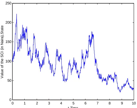
is the volatility arising from the stock market. Fi- gure 1 presents the simulated diffusion paths of (7).
Figure 1 was obtained by setting k0.099,
1 0.25
D
, 2 0.36, ,
D
D0100 0
t t
dt nt
, t10,
0 0
t and nt1000.
Applying Itoˆ lemma to (7), we obtain
2
0
1
exp .
2 D D
D t D k t W t
0 1 2 3 4 5 6 7 8 9 10 0
50 100 150 200 250
V
a
lue
of
t
h
e
S
C
I
(i
n
N
a
ir
a)
,S
ta
te
t,Time
Figure 1. Simulated diffusion paths of the stochastic cash inflows.
4. The Wealth Process
Let X t
be the wealth process and
t
I
t , S
t
be the portfolio value at time , twhere is the portfolio value in inflation-linked bond and is the portfolio value in stock at time t. Then,
I t
S
t
t
t
0
t 1 I S is the portfolio value in cash account at time . Therefore, the dynamics of the wealth process is given by
t
( ) ( )
, ,
1
0 .
S
I
I S
dS t
dX t X t t
S t
dB t I t
X t t
B t I t
dQ t
,
X t t t D t
Q t
X x
dt
(9)
Substituting (1), (2) and (3) into (9), we obtain
,
0 .
dX t X t r t D t dt
X t t dW t
X x
(10)
5. The Discounted Value of SCI
In this section, we determine the value of expected discounted SCI.
Definition 1:
The discounted value of the expected future SCI is defined as
t tT
d ut E D t u
t
(11)where, EtE
|Ft
is the conditional expectation with respect to the Brownian filtration
Ft t0 and
t Z t
exp
rt is the stochastic discount factor which adjusts for nominal interest rate and market price of risks for stock and inflation-linked bond.
Proposition 1:
Suppose
t is the discounted value of the ex- pected future SCI, then
exp
D
1
. DD t k r T t
t
k r
(12)
Proof. By definition 1, we have that
t tT
du D u
t D t E u
t D t
(13)Applying change of variable on (13), we have
=
0
d0 0
T t D
t D t E
D
(14)Applying parallelogram law and martingale principles on (14), we have
0 0 exp
D
. DE k r
D
Therefore,
0 exp
d .
T t
D
t D t k r
(15)Integrating, we have
exp
D
1
. DD t k r T t
t
k r
(16)
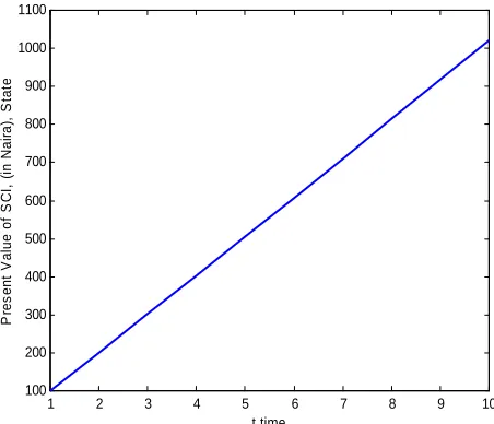
Figure 2 was obtained by setting , k = 0.099,
r = 0.04, , ,
0 100
D
0.09
1 0.25
D
2 0.36
D
, S 0.4,
0.3
I
, 0.6 and I 0.08.
At t0, we obtain the present discounted value of
future SCI to be
0
0
exp 1
0 D .
D
D k r T
k r
(17)
If r D k and we allow T i.e.,
0 0
exp 1
lim lim D ,
T T
D
D k r T
k r
0 , .
D
D D
r k
D
r k
r k
[image:3.595.59.287.85.264.2]1 2 3 4 5 6 7 8 9 10 0
200 400 600 800 1000 1200
P
res
en
t V
al
ue
of
S
C
I,
(
in Nai
ra)
, S
tat
e
[image:4.595.310.536.85.279.2]t,time
Figure 2. The flow of the discounted value of SCI.
0 0
exp 1
.
D k r T
k r
(18)
Hence,
0 0
0
exp 1
lim lim ,
, .
T T
D k r T
r k k r
D r k r k
This shows that as T , 0 converges to
0
D D
r k, provided r D k.
For the deterministic case, it shows that as T ,
0
converges to D0
rk, provided rk.
Figure 3 was obtained by setting , k = 0.099,
r = 0.04, , ,
0 100
D 0.09
1D 0.25
2D0.36 , S 0.4,
0.3 I
, 0.6 and I 0.08.
Figure 2 represents the flow of the discounted value of stochastic cash inflow in the investment at time and Figure 3 represents the present value of discounted future SCI at time
t
.
t
We now consider the sensitivity analysis of 0. Pro- position 2 establishes this fact.
Proposition 2:
Let k r D , then
0
0exp .
D T
T
Proof. The results follow by taking the partial deri- vatives of 0 with respect to T, D0, r, D and
, respectively.
k
0 0
0 0
1 1
1 ;
D D T
1 2 3 4 5 6 7 8 9 10
100 200 300 400 500 600 700 800 900 1000 1100
Pr
e
s
e
n
t Va
lu
e
o
f SC
I,
(
in
N
a
ir
a
),
St
a
te
[image:4.595.60.286.86.279.2]t,time
Figure 3. The present discounted value of future SCI.
0 0
0 2
1
1 T D ;
r T
0 0;
D r
0 0
0 2
1
1 .
T D
k T
0 r
[image:4.595.336.508.317.409.2]
Table 1 shows the sensitivity analysis of the dis- counted value of the SCI.
Proposition 3:
Suppose that Proposition 1 holds, then
.D D
d t t r dt dW t
D t dt
(19)
Proof. Finding the differential of both sides of (16) and then substitute (7), we have
exp 1
exp
exp 1
exp 1
exp 1
. D
D
D D
D D
D t T t
d t kdt dW t
D t
T t dt
D t
T t kdt dW t
T t dt D t dt
D t T t
r dt dW
D t dt
t r dt dW t D t dt
t
Table 1. Simulation of the sensitivity analysis.
T 0
0
D
10
D
20
D
T0
r0
0
I
S0
k0
1 1.0022 −16624 −20005 0.4359 −207850 −51962 −74826 207850
2 2.0087 −14857 −17875 0.8738 −185720 −46429 −66858 185720
3 3.0197 −13079 −15736 1.3136 −163490 −40872 −58855 163490
4 4.0350 −11293 −13587 1.7552 −141160 −35290 −50818 141160
5 5.0548 −9499 −11429 2.1988 −118740 −29685 −42746 118740
6 6.0790 −7697 −9261 2.6444 −96220 −24054 −34638 96220
7 7.1077 −5888 −7084 3.0918 −73600 −18400 −26495 73600
8 8.1408 −4070 −4897 3.5413 −50880 −12720 −18317 50880
9 9.1785 −2245 −2701 3.9926 −28060 −7016 −10103 28060
10 10.2207 −412 −495 4.4460 −5150 −1287 −1853 5150
V t as
:
V t X t t , (20) where, X t
satisfy (10) and
t satisfy (19).Proposition 4:
Let V t
satisfy (20), X t
satisfy (10) and
t satisfy (19), then
.D
D
dV t
r X t t X t t dt
X t t t dW t
(21)
Proof. Finding the differential of both sides of (20) and then substitute in (10) and (19), the result follows.
6. Optimization of the Value of Wealth
Process
We define the general value function
,
,
,
,
J t v E u V t X t t X t x t
where u V t
is the path of V t
. Define to be the set of all admissible portfolio strategy that are F-pro- gressively measurable, that satisfy the integrability con- ditions T
d and lett
E u u u
U V t
bea concave function in V t
such that satis- fies the HJB equation
U V t
, sup | ,
, sup
U t v E u V T X t x t
J t v
, (22)
subject to:
, 1 , 1v U T v
where,
2
2
1 2 1
2
x D x
D x x
D D
HV r U rxU U x t U
x
x t U x t t U
U
(23) Let U t v
,he utility ooth,
be the solution of the HJB equation (22). Since t function is concave and the value f tion is sm
unc- i.e., U t V
, C1,2
R
0,T
, then (22) is well-defined. Hence, we have the following:
x
xx DHV
U x t U U
t
0
X
(24)
from (24), we have
1
1.
D x
x
xx xx
U U
xU xU
t
(25)
Substituting (25) into (22), we obtain the foll HJB equation:
owing
2
1
t x
U rxU
1
2 2 2 2
1
2
2 2
0.
D D D
x D D x
xx xx
D x x
xx
r U U
U U
U U
U U
U
(26)
This is the resulting HJB equation of our problem. Therefore, by applying Itô lemma on (21), we obtain
the following HJB equation:
, max 0t
U t v HV
Proposition 5:
The solution of the HJB equation (26) is of the form
1
, , 0, 0,
1 vA t U t v
with
1.exp ,
2
A t r T t
(27)
A T
Proof. Finding the partial derivatives of
1
,
1 vA t U t v
with respect to t,
x, xx, ,
x an
the follo
d and then substitute into (26), we obtain wing:
1 1 1 1 1 2 1 0. 2v A t A t rv A t
v A t
(28)
From (28), we obtain
exp , 2 0 1A t r Tt
A
Using (29), we obtain
(29)
1
, exp 1
1 2
1 v
U t v r T
(30)
Figure 4 was obtained by setting
1
, v .
U T v , t 0 100
D , r0.04, 0.6
0.099
k , T 10, 1 0.25
D
, 2 0.36
D
, ,
0.09
, S 0.4, I 0.3 and I 0.08 e of utility of
. wealth Figure 4 shows the expected valu
at time t
0,10
for different values of . Here, measures the l vel of risk the investor is willing to take. Obse aller the value ofe
rve that the sm , th ig expecte of wealth, and vice vers Theref when e h a. her the d value 0.07 ore,
, the expected value of utility of wealth,
t v, U
10,v
2780.9, when 0.08U ,
10,v
2271.5, when 0.09U , U
10,v
n
1914.
1
and whe 0.10 at which i
, U ,v 8 . the
nv
sk more0 ors are 1 est 164 ri .7 av H erse, ence, the lower the rate
th
e
e wealth that will accrue to them, and vice versa, which is an intuitiv result.
Proposition 6:
Suppose that U t V
, is the solution of the HJB Equation (26), then the optimal portfolio in inflation- linked bond, stock and cash account are given by
1 2 3 4 5 6 7 8 9 10
0 500 1000
1 D t . I I I V t tX t X
t
(31)
1500 2000 2500 3000 E x p e c ted U t lt h (i n
Time,t (in year)
il it y of Wea N a ir a)
[image:6.595.309.538.85.261.2]Expected Wealth for Gamma=0.07 Expected Wealth for Gamma=0.08 Expected Wealth for Gamma=0.09 Expected Wealth for Gamma=0.10
Figure 4. The expected value of utility of wealth for diffe- rent values of γ.
2 2 2 2 1 2 1 1 . 1 SI I S S I
I S D D I S I S t r V X t t X t t (32)
0 t 1
2 2 2 2 1 1 2 1 1 . 1
I I S S I
I
I S
D D
D
I S
I I S
r V t X t t X t
Proof. From (25), we have that
1
2 1
.
D
V t t
t
X t X t
But, 1 1 2 1 2 1 D I
D D D
I S S I
2 2 2 2 1 1 I II S I S
[image:6.595.63.292.101.470.2] [image:6.595.313.537.304.748.2]Therefore,
1 2 2 1 2 2 2 1 2 2 2 1 1 1 1 1 D I I I I D DI S I S I I S
S S I S I D I I I
I S I S I I
S I
V t t
t t
r
t X t X t
V t t
X t X t
r V t
X t
2 1 2 1 2 2 12 2 2
1 1 1 1 D D S S I D I I I D D
I S I S I I S
S I S I
t
X t
V t t
X t X t
r V t t
X t X t
It implies that
1
. D II
I
V t t
t
X t X t
(33)
2 2 2 2 1 2 ( ) 1 1 . 1 SI I S S I
I S D D I S I S t r V X t t X t t (34)
0 2 2 2 2 1 1 2 1 1 1 . 1 II I S S I
I S
D D
D
I S
I I S
V t t X t r V X t t t
X t X t
t (35) From (33), the first term represents the classical port- folio strategy while the second term represents the inter- temporal hedging strategy that offset any shock to the SCI at time t. From (34),
2 2 2 1 1I I S S I
I S r V X t t represents
the classical portfolio strategy at time t and
2 1 2 1 D D I S I S t X t represents the intertemporal
hedging term that offset shock resulting from the SCI at time . From (35), observe that these hedging terms can be tra sfer to cash account at time or it can be rein- vest in stock and in inflation-linked b d at time
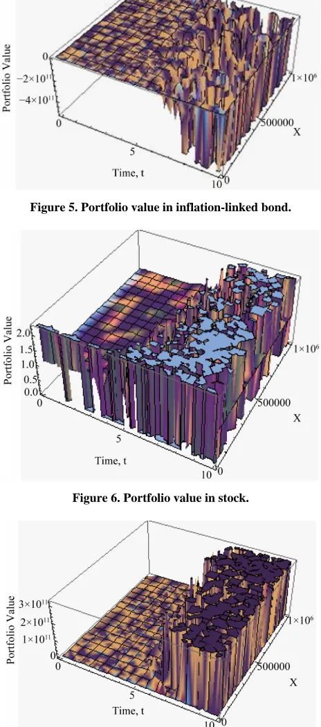
Figure 5 was obtained by setting ,
t
n t
on t.
0 100
D r0.04,
0.099
k , T 10, 1 0.25
D
, 2 0.36
D
, 0.6,
0.09
, S 0.4, I 0.3, I 0.08 and 0.5. The optim
time t 10
al portfolio value in inflation-linked bond at
[image:7.595.63.454.87.649.2] is obtained as
Figure 6 was obtained by setting , 0.16 (or 16%).
0 100
D r0.04,
0.099
k , T 10, 1D 0.25, 2D0.36, 0.6,
0.09
, S 0.4, I 0.3, I 0.08 and 0.5.
10
t
The optimal portfolio value in stock at time is obtained as 1.001562 (or 100.1562%).
Figure 7 was obtained by setting D0100, r0.04,
0.099
k , T 10, 1D 0.25, 2D0.36, 0.6,
0.09
, S 0.4, I 0.3, I 0.08 and 0.5. ount at time The optim
10
t
al portfolio value in cash acc
is obtained as −0.161562 (or −16.1562%). In Figures 5-7, we set D0100, r0.04, k0.099,
10
T , 1D 0.25, 2D 0.36, 0.6, 0.09,
0.4
S
, I 0.3, I 0.08 and 0.10. Figure 5 shows the portfolio value in inflation-linked bond. We found that the optimal portfolio value in inflation-linked bond at time t10 is 0.16 (or 16
at time t
%). Figure 6 We found that
10 is 1.
shows the optimal 001562 (or the portfolio
portfolio
value in stock.
lio d b Figure 5. Portfo value in inflation-linke ond.
val k.
Figure 6. Portfolio ue in stoc
Figure 7. Portfolio value in cash account.
account. We found that the optimal portfolio value in cash account at time t = 10 is −0.161562 (or −16.1562%).
7. Conclusion
The astic
sh inflows was considered. It was assumed that the cash
inflow, stock and inflation-linked bond are stochastic and follow a standard geometric Brownian motion. The sen- sitivity analysis of the present value of the discounted cash inflows was carried out in this paper and the results are presented in Table 1. Analytical solution to the resulting HJB equation was obtained. It was found that the smaller the value of
optimal portfolio strategy X with discounted stoch ca
(which measure the level of risk the investor is willing to take), the higher the expected value of wealth, and vice versa. The optimal portfolio values in stock, inflation-linked bond and cash account were ob- tained. The resulting optimal portfolio values in stock and inflation-linked bond were found to involve intertem- poral hedging terms that offset any shock to the SCI.
REFERENCES
G. Dee Optimal In-
vestment Strategies in a CIR Framework,” Journal of Applied Probability, Vol. 37, No. 4, 2000, pp. 936-946. doi:10.1239/jap/1014843074
[1] lstra, M. Grasselli and P. Koehl, “
[2] D. O. Cajueiro and T. Yoneyama, “Optimal Portfolio, Optimal Consumption and the Markowitz Mean-Variance Analysis in a Switching Diffusion Market,” 2003. unb.br/face/eco/seminarios/sem0803.pdf
[3] A. Zaks, “Present Value of Annuities under Random Rates of Interest,” 2003.
http://academic.research.microsoft.com/Publication/624417 5/present-value-of-annuities-under-random-rates-of-interest [4] D. Dentcheva and A. Ruszczynski, “Portfolio Optimi-
zation with Stochastic Dominance Constraints,” SIAM Journal on Optimization, Vol. 14, No. 2, 2003, pp. 548-
566. doi:10.1137/S1052623402420528
[5] D. B lio Insur-
ance: An Analysis of Financial Asset Portfolioslake, “Efficiency, Risk Aversion and Portfo Held by Investors in the United Kindom,” Economic Journal, Vol. 106, No. 438, 1996, pp. 1175-1192. doi:10.2307/2235514
[6] A. Zhang, “Stochastic Optimization in Finance and Life lications of the Martingale Method,” Ph.D. ity of Kaiserslauten, Kaiserslautern, 2007.
fined
tical Finance, Vol. 2, No. 1, 2012, pp. 132-139.
doi:10.4236/jmf.2012.21015
Insurance: App Thesis, Univers
[7] J. Mukuddem-Peterson, M. A. Peterson and I. M. Schoe- man, “An Application of Stochastic Optimization Theory to Institutional Finance,” Applied Mathematics Sciences,
Vol. 1, No. 28, 2007, pp. 1359-1385.
[8] P. Battocchio, “Optimal Portfolio Strategies with Sto- chastic Wage Income: The Case of a Defined Contribu- tion Pension Plan,” Working Paper, Uni sité Catholique de Louvain, Louvain-la-Neuve, 2002.
[9] B. H. Lim and U. J. Choi, “Optimal Consumption and Portfolio Selection with Portfolio Constraints,” Interna- tional Sciences, Vol. 4, 2009, pp. 293-309.
[10] C. I. Nkeki, “On Optimal Portfolio Management of the Accu- mulation Phase of a Defined Contributory Pension Scheme,” Ph.D. Thesis, University of Ibadan, Ibadan, 2011.
[11] C. I. Nkeki and C. R. Nwozo, “Variational Form of Classi- cal Portfolio Strategy and Expected Wealth for a De Contributory Pension Scheme,” Journal of Mathema-