Approximate Reasoning in Fuzzy Resolution
Banibrata Mondal, Swapan Raha
Department of Mathematics, Visva-Bharati University, Santiniketan, West Bengal, India Email: mbanibrata@gmail.com, swapan.raha@visva-bharati.ac.in
Received January 2, 2013; revised February 3, 2013; accepted February 20, 2013
Copyright © 2013 Banibrata Mondal, Swapan Raha. This is an open access article distributed under the Creative Commons Attribu-tion License, which permits unrestricted use, distribuAttribu-tion, and reproducAttribu-tion in any medium, provided the original work is properly cited.
ABSTRACT
Resolution is an useful tool for mechanical theorem proving in modelling the refutation proof procedure, which is mostly used in constructing a “proof” of a “theorem”. An attempt is made to utilize approximate reasoning methodol- ogy in fuzzy resolution. Approximate reasoning is a methodology which can deduce a specific information from general knowledge and specific observation. It is dependent on the form of general knowledge and the corresponding deductive mechanism. In ordinary approximate reasoning, we derive B from A→B and A by some mechanism. In inverse approximate reasoning, we conclude A from A→B and B using an altogether different mechanism. An important observation is that similarity is inherent in fuzzy set theory. In approximate reasoning methodology-similarity relation is used in fuzzification while, similarity measure is used in fuzzy inference mechanism. This research proposes that simi-larity based approximate reasoning-modelling generalised modus ponens/generalised modus tollens—can be used to derive a resolution—like inference pattern in fuzzy logic. The proposal is well-illustrated with artificial examples.
Keywords: Approximate Reasoning; Similarity Index; Similarity Based Reasoning; Resolution Principle
1. Introduction
In automated theorem proving, resolution is a rule of inference leading to a refutation theorem-proving tech- nique. Applying the resolution rule in a suitable way, it is possible to check whether a propositional formula is satisfiable and construct a proof that a first-order formula is satisfiable/unsatisfiable. In 1965, J. A. Robinson [1] introduced the resolution principle for first-order logic. A resolvent of two clauses containing the comple- mentary literals and respectively, is defined as
2
is understood as the disjunction of the literals present in them. It is also a logical consequence of 1
1, 2
C C p
C p
1
1, 2
,res C C C p p
∪
∪
2
C C . A resolution deduction of a clause C from a set S of clauses is a finite sequence of clauses C C1, 2, , CnC
S
UE
such that, each Ci is either a member of or is a
resolvent of two clauses taken from From the resolution principle in propositional logic we deduce that, if is true under some truth valuation , then v(Ci) =
TRUE for all i, and in particular, [2]. .
S
v
TR
S
v C
Example 1: Here, is a derivation of a clause from a set
[image:1.595.324.523.431.559.2]of clauses presented by means of a resolution Tree in Figure 1.
In first order logic, resolution condenses the traditional syllogism of logical inference down to single rule. To
Figure 1. Resolution Tree. A simple resoluion scheme is:
premise1 : premise2 : conclusion :
a b
b a
recast the logical inference using the resolution technique, first the formulae are represented in conjunctive normal form. In this form, all quantification becomes implicit: universal quantifiers on variables are simply omitted as understood, while existentially quantified variables are replaced with Skolem functions.
X Y, ,
was taken by Lee and Chang [3]. Lee’s works [3,4] were continued and implemented by many researchers. Lee’s fuzzy formulae are syntactically defined as classical first-order formulae, but they differ semantically as the formulae have a truth value in [0,1]. An interpretation I is defined by an assignment TI of a truth value to each
atomic formula, from which truth values of compounded formulae are computed [5]. Interpretation I is said to satisfy (or falsify) a formula F, if TI
, the truth value ofF
F under I, is at least 0.5 (or at most 0.5). A formula is said to be unsatisfiable if and only if, it is falsified by all its interpretations. A set of clauses is unsatisfiable in fuzzy logic if and only if, it is unsa- tisfiable in binary logic [3]. Mukaidono [6,7] has gene- ralized Lee’s result in the following way:
S
For two clauses C C1, 2 in fuzzy logic, let
, AL
1 1 2 2 where 1 and 2 do not
contain the literal
in approximate reasoning.
,
C A L C L L
A and A
respectively as a factor and have no pair of complementary variables. Then the clause 1 2 is said to be a classical resolvent of
1 2 written as 1 2 whose keyword is
L L
,
C C R C C
, A andthe contradictory degree of the keyword is
A1 C2
1,C2
S cd R C
R C
. A fuzzy resolvent of 1 2 is written as cd
where is the contradictory degree of the keyword or the confidence associated with the resolvent. They have computed the truth value of cd from the truth value of 1 2 and the truth values of the atomic formulae. Then, it is proved a set of fuzzy clauses is unsatisfiable if and only if, there is a deduction of empty clause with its confidence of resol- vent from Dubois and Prade [8] established fuzzy resolution principle in the case of uncertain proposition. In [9], antonym-based fuzzy hyper-reso- lution was introduced and its completeness was proved. S
nchez et al. [10] proposed a fuzzy temporal con- straint logic and introduced a valid resolution principle in order to explain/clarity some queries in this logic. Fontana and Formato [11] introduced a fuzzy resolution rule based on an extended most general unifier supplied by the extended unification algorithm. S. Raha and K. S. Ray [12] presented a generalised resolution principle that handles the inexact situation effectively and is applicable for both well-defined and undefined propositions. They associated a truth value to every proposition. We assume the fuzzy propositions to be completely true and, hence, do not associate partial truth value to the propositions. Our idea is to present, a generalised resolution principle that deals with the fuzzy propositions by the technique of inverse approximate reasoning. The advantage is that, it executes effective resolution and shows its flexibility for automated reasoning. To avoid the generic problem in handling generalised modus ponens (GMP) we use inverse approximate reasoning in fuzzy resolution. We also define fuzzy resolution on the basis of similarity/ dissimilarity measure of fuzzy sets, which is inherent
,
C C
cdcd A
0
cd S.
a
, ,
,
1
,R C C
Let us consider two clauses C1 P C and
2
C PC2. Resolvent of C1 and C2 denoted by
1, 2
res C C C1C2
P
if and only if similarity between and
not P is greater than or equivalently, dissimilarity between and is less than
P
P 1,
being pre-defined threshold. Instead of complementary literal, we introduce similar/dissimilar literal here. The argument form of simple Fuzzy Resolution is as follows.
A B
notB A
The scheme for Generalised Fuzzy Resolution is given in Table 1.
In this case, we can say that the Disjunctive Syllogism holds if B is close to notB, A is close to A.
The scheme in Inverse Approximate Reasoning looks like as given in the following Table 2.
Here, fuzzy sets A and A are defined over the universe of discourse U
u1, ,u2 ,um
and fuzzy setsand
B B are defined over the universe of discourse
, n
.V v1, ,v2 v
We shall transform the disjunction form of rule into fuzzy implication or fuzzy relation and apply the method of inverse approximate reasoning to get the required resolvent. However, in the case of complex set of clauses the method is not suitable. Hence, we investigate for another method of approximate reasoning based on similarity to get the fuzzy resolvent.
This paper consists of eight sections. In Section 2, we define and dicuss some basic concepts which are used in our paper. We briefly describe two methods of inverse approximate reasoning proposed in [13], in Section 3, and apply the method of inverse approximate reasoning towards fuzzy resolution in Section 4. Another method for fuzzy resolution in the case of complex clauses, is applied in Section 5. Section 6 is devoted with some artificial examples to illustrate the method. At last, in Section 7 some conclusions are made, follwed by some references.
Table 1. Generalised fuzzy resolution. Rule: X is A or Y is B
Fact: Y is B
Conclusion: X is A
Table 2. Inverse approximate reasoning. Rule (p): If X is A then Y is B
Fact (q): Y is B
2. Preliminaries
To study ordinary approximate reasoning as well as inverse approximate reasoning, we have to deal with fuzzy sets, fuzzy relations and operations on fuzzy sets, fuzzy connectives not
, and
and or
. These are represented by the well known classes of negation functions (to model complement operators), continuous triangular norms (t-norms to model conjunc- tion) and triangular conorms (t-conorms to model dis- junction) respectively.Some well-known t-norms and correlated t-conorms are listed in Table 3, where M, P, B indicate minimum, product, bounded product and drastic product respec- tively for t-norms, and maximum, algebraic sum and bounded sum respectively, for the correlated t-conorms.
Typically, a fuzzy rule “If X is A then Y is ” (
B A and B are fuzzy sets) is expressed as I a b
, , where I is a fuzzy implication and a and are membership grades ofb A and respectively. From an algebraic point of view, some implication operators basically identified in [14] are classified with four
families , where 1
B
1,2,3,
, T i
I i 4 I , known as QL-
implication, is based on classical logic form
and logical operators are substituted by fuzzy operators. Family 2
a ab
a
a
b
I , often named S-implication, derives from classical logic form
Families 3
. b
a b a I and I4 reflect a partial ordering on propositions and are based on a gene- ralisation of modus ponens and modus tollens, respec- tively. Family I3 is known as R-implication. With
reference to the t-norms and t-conorms in Table 3, the explicit expressions of fuzzy implication operators T
i
I are presented in Table 4.
Table 3. t-norms and t-conorms.
T T T a b , T a b,
M min , a b max , a b
P a b a b a b
[image:3.595.58.284.608.731.2]B max 0, a b 1 min 1, ab
Table 4. Expression of fuzzy implication operators.
T
i
I M P B
1 T
I max min , ,1
a b a
1 a a b2 max 1 a b, 2T
I max 1 a b, 1 a a b min 1 a b,1
3 T
I 1 if
otherwise
a b
b
1 if
otherwise
a b
b a
min 1 a b,1
Here, some of the most popular implications such as the Kleene-Dienes, Reichenbach, Lukaseiwicz, Gödel and Gaines implication operators correspond to
2 , 2, 2, 3 3
M P B M P
I I I I and I respectively.
The notion of similarity plays a fundamental role in theories of knowledge and behaviour and has been dealt with extensively in psychology and philosophy. If we study the behaviour pattern of children we find that, children have a natural sense to recognize regularities in the world and to mimic the behavior of competent members of their community. Children thus make deci- sions on similarity matching. The similarity between two objects suggests, the degree to which properties of one may be inferred from those of the other. The measure of similarity provided, depends mostly on the perceptions of different observers. Emphasis should also be given to different members of the sets, so that no one member can influence the ultimate result. Many measures of simi- larity have been proposed in the existing literature [15,16]. A careful analysis of the different similarity measures reveals, that it is impossible to single out one particular similarity measure that works well for all purposes.
Suppose U be an arbitrary finite set, and F(U) be the collection of all fuzzy subsets of U. For A B,
U , a similarity index between the pair {A,B} is denoted as S(A,B;U) or simply S(A,B) which can also be consi- dered as a function S:
U
U
0,1 . In order to provide a definition for similarity index, a number of factors must be considered. We expect a similarity measure S A B
,
to satisfy the following axioms:P1. S B A
,
,S
AB
, S not A, not ,B
S A B
, not A being some negation of A.P2. 0S A B
,
1.P3. S A B
,
1 if and only if A B.P4. For two fuzzy sets A and , simultaneously not null, if
B
,
0S A B then min
A
u ,B
u
0 for all u U , i.e., AB .P5. If either A B C or A B C then
,
m
,C
S A C in S A B S, , B .
A similarity measure between two fuzzy sets satisfying these axioms can also be termed as a f-near-degree. For
0 1, if S A B
,
, we say that the two fuzzy setsA and are -similar. We now consider a defi- nition of measure of similarity which has been proposed in [17,18].
B
4 T
I 1 if
1 otherwise
a b
a
1 if
1
otherwise 1
a b a b
min 1 a b,1
Definition 1—Similarity Indices: Let A and be two fuzzy sets defined over the same universe of dis- course The similarity index of pair
B
.
U S A B
,
A B,
is defined by
1
1
, 1 A B q q
u
S A B u u
n
where is the cardinality of the universe of discourse and is the family parameter. Here, is a real number such that a large always gives a large similarity measure. It is left to the user to set for a problem. It is easy to say that the similarity measure referred to in the Definition 1 satisfies axioms P1, P2, P3, P4 and P5.
n
1
q q
q
q
,
S A B S A C,
implies that “ is at least as close toB
A as C is to A”. as given in Definition 1 is quite sensitive-every change in
,
S A B
A or will be reflected in . Detailed clarification of choice of the definition is described in [18].
B
,S AB
Measure of dissimilarity is another measure of com- parison of objects in literature. Many authors like B. Meunier et al. [15] have defined measure of dissimi- larity in different way. However, we use the dissimilarity measure in the context of similarity measure and consider measure of dissimilarity of two fuzzy subsets
A and defined over B
U , denoted by D A B
,
as Moreover, we assume
Through out the paper, we use this concept of dissimilarity. In the next section, method of inverse approximate reasoning is discussed briefly.
,B
1
,D A S A B
,
not ,
D A B S A B
.
, notS A B
.3. Inverse Approximate Reasoning
Let there be a fuzzy rule: “If 2 flow rate is LOW then
heating power is LOW”. Let us suppose that the “heating power is rather LOW”. Then, by the method of inverse approximate reasoning with a single rule, we may construct hypotheses which would explain the causes of observation by fuzzy mathematical method. Let us consider a second example as considered in [19]. Let there be two fuzzy rules: “if the traffic is crowded then the flow is low” and “if the visibility is weak then the flow is low”. Suppose, we observe “the flow is very low”. According to these two linguistic rules and the corre- sponding observation, we first construct hypotheses by abduction such as “the traffic is very crowded” or “the visibility is very weak” or “the traffic is very crowded and the visibility is very weak”. It is difficult to decide which are possible explanations for this observation. N. Mellouli and B. Bouchon-Meunier [20] have used gene- ralised modus ponens (GMP) to construct abductive hypotheses and used the measure of similitude to con- struct the best possible explanation. Here, we consider a single rule for the method of inverse approximate rea- soning.
O
Definition 2—Inverse Approximate Reasoning: Let : If X is AthenY is
p B (1)
be a given rule, where A and are fuzzy subsets defined over the universes of discourse U and V respectively. From a given fact “
B
X is A”, where A
is a fuzzy subset of U we can conclude that “Y is B”, where B is a fuzzy subset of V , by applying some method of approximate reasoning. This is called forward approximate reasoning. Now for given “Y is B”, we consider
B be the set of all fuzzy subsets A of U such that for given “X is A” we can conclude “ is Y B” by the method of approximate reasoning. We have to choose the best member/s of
B (not empty) in some sense and define some inverse mapping from fuzzy subsets of V into fuzzy subsets of U , which we refer here as inverse appro- ximate reasoning. We shall discuss briefly two methods of inverse approximate reasoning presented in [13] to establish fuzzy resolution principle.
3.1. Similarity Based Inverse Approximate Reasoning
Our aim, in [13], was to feed the method of similarity- based approximate reasoning [17] to inverse approximate reasoning by writing the rule into its equivalent form. Let X , be two linguistic variables and , be their respective universes of discourse. Two typical propo- sitions “p” and “q” are given in scheme as presented in Table 2 and we may derive a conclusion according to similarity based inference method [17] of the scheme in Table 2. The membership values of
Y U
, , V
A A B and B are defined as before. Unlike the existing similarity based methods, a convenient way to represent a rule given by premise “p” is in the form of a fuzzy relation. The rule in premise “p” may be transformed into its equivalent form “ p” of the given premise “p”. We represent this equivalent rule by a fuzzy relation R
0,1V U [21]. Usually, is defined on the basis of one of the operationR
, ,
, where is
associative, commutative and the conjunction operator in the GL-monoid
2: 0,1
0,1
0,1 , , . is the residuation ope- ration associated with the conjunction and can be viewed as the valuation function for the implication;
is an alternative to the lattice operation (in this case simply the “min” operation) for the valuation of the conjunction. Then for a given fact, the similarity between the fact and the antecedent of the equivalent form of the given rule denoted by “p” is computed and is used to modify the relation . Here, every change in the concept, as it appears in the conditional equivalent premise and in the fact, is incorporated into the induced fuzzy relation (say,
R
R). The conclusion may then be drawn using the projection operation, valuating the existential quantifier by the supremum and the conjunction by the operation . We obtain the definition of the composition of a fuzzy relation and a fuzzy set as
,
,
,A u v V R v u B v u
U.
In order to avoid the use of rule-misfiring, we modify the inference scheme in such a way that significant change will make the conclusion less specific. This is done by choosing an expansion type of inference scheme. Here, the “UNKNOWN” case, i.e., the fuzzy set AU , is to be taken as the limit of non-specificity. Explicitly, when the similarity value becomes low, i.e., when
and differ significantly, the inference should be
not B B
.
AU
not
As for B not B, we expect that A A and for all other B, the relation Anot A holds. This in turn implies that, nothing better than what the rule says, should be allowed as a valid conclusion. In view of the above observation we propose a scheme for computation of A in the following algorithm.
ALGORITHM-SIAR:
Step 1. Translate given premise and compute using some suitable translating rule (possibly, a t-norm).
p
not , notR B A
Step 2. Compute similarity measure S
not ,B B using some suitable definition .Step 3. Modify R
not , not B A
with S
not ,B B
to obtain the modified conditional relation
not , not
R B A B using some scheme C. Step 4. Use sup-projection operation on
not , not
R B A B to obtain A as
sup
not ,not
, .A u v R B A B v
u (2)
In [17,18], authors have proposed two schemes for computation of the modified conditional relation
not , not
R B A B as given in Step 3, the general form of which is given by:
Scheme C:
not ,not
,
Rnot ,not B A
R B A B v u s v u
,
,
where is any implication function. As previously done in [13], We have
supv V Rnot ,not B A
,A u s v u
(3)
and when the conditional relation is interpreted as a t-norm we get
not A
.A u s u
Otherwise, A by SIAR could be anything. From (2) and (3) it is found that when we have
.
not , 0
S B B
AU In other words, it is impossible to conclude any- thing when
not ,B B
are completely dissimilar, i.e.,
B B,
are completely similar. When S
not ,B B
is c l o s e t o u n i t y, R
not , not B AB
i s c l o s e t o. Hence, the inferred fuzzy set
not ,not
R B A A will
be close to not A, i.e., is close to unity. Scheme also ensures that a small change in the input
produces a small change in the output and hence, in this
not ,S A A
Csense the above mechanism of inference is reasonable. Let us consider the model as in Table 2 and a theorem is established as follows:
Theorem 1: For all notB and B, not .AA We have investigated another method to deal with fuzzy implication operators in inverse approximate rea- soning.
3.2. Method Using Cylindrical Extension and Projection—INAR
We now consider the scheme given in Table 2 and inves- tigate the scheme for generalised modus tollens (GMT). We describe the method simply by an algorithm.
ALGORITHM-INAR:
Step 1. Translate the rule into a fuzzy relation or implication operator R.
Step 2. Take the of fuzzy sub- set
cylindrical extension
B in V on U V and let it be R.
Step 3. Construct R R∩R , where is defined by any fuzzy conjunction operator.
∩
Step 4. Obtain A proj R on U. Symbolically, we get,
v V
,A u proj R u v
, , ,
,supv V T R u v R u v
T is a t-norm
, ,
supv V T B v R u v
,
by definition of cylindrical extension, which establishes the CRI in the form of GMT. We have to select an appropriate fuzzy implication for the fuzzy relation in Step 1 so as to model GMT. Also the standard negation of the resulted fuzzy set obtained by GMT also gives the given observation by applying GMP. Hence, mathe- matical formulation of the above algorithm is:
sup
, R
,
A B
v V
u T v u v
. (4)
We now deduce some theorems from which we can establish the reasonableness of the method in which negation operator is taken as standard strong negation.
Theorem 2: Let B be normal and .
Then
not
B B not AA, whenever the following implications satisfy the Equation (4) for any t-norm T:
1) Reichenbach S-implication; 2) Kleene-Dienes S-im- plication and 3) Lukasiewicz R and S-implication.
Theorem 3: Let B be normal and .
Then , whenever both the relation
and conjunction in the Equation (4) are defined by any t-norm .
not
B B
UNK
A T
NOWN
Theorem 4: Let B be normal and .
Then
not
B B
Theorem 5: Let be normal and .
Then
B Bnot B
not AA, if A
u 0.5 and not AA, if
0.5A , whenever Gödel R-implication and Gou-
gen R-implication satisfy the Equation (4) for any t-norm T.
u
We observe in the above theorems that if then either
not
B B A will be not A or close to not A, that is, we may use GMT in the case of inverse approximate reasoning to get an output in the antecedent part of the given rule and the negation of this output may give B by applying GMP. So, we first consider the similarity between and . If the similarity measure between these two is very very low, i.e., then we expect similarity between
B B
,S B B
0 A and A
,S B B
to be very low, i.e., . If the similarity measure between these two is very very high, i.e., then we cannot make any specific conclusion about the similarity between
S A,A 0
1A and A. Therefore, the method of inverse approximate reasoning demands dissimilarity between the specific observation and the consequent of the given rule. So we can apply the method in fuzzy resolution.
4. Fuzzy Resolution Based on Inverse
Approximate Reasoning
Lately researchers discuss and explore the validity of many classical logic tautologies in fuzzy logic, especially those that involve fuzzy implications. We attempt to exploit such a classical logic equivalence to deal with fuzzy resolution in the framework of inverse approximate reasoning methodology. In classical logic
, , 0,1 .
a b a b a b (5) when extending this classical logic equivalence to fuzzy logic, we interpret the disjunction and negation as a fuzzy union (t-conorm) and a fuzzy complement, res- pectively. Fuzzy implication thus obtained is usually referred to in the literature as S-implication.
We now consider the classical logic tautology which is obtained from (5).
, , 0,1 .
a b a b a b (6) Therefore, we can extend the classical equivalence (6) into fuzzy logic where fuzzy union is transformed to fuzzy implication.
In fuzzy resolution we deal with the rule of the type “X is A or Y is B”. Like classical logic, we may trans- form the rule into “If X is not A then Y is ” into fuzzy logic. Then the rule is executed in the method of Inverse Approximate Reasoning described in [13] to obtain the disjunct. The equivalent scheme of Table 1 that conforms fuzzy resolution is given in the Table 5.
B
[image:6.595.308.537.102.153.2]We have demonstrated earlier in [13] that—if the give
Table 5. Equivalent scheme conforms fuzzy resolution.
Rule: If X is notA then Y is B
Fact: X is B
Conclusion: X is A
iven rule then one may conclude that the resulting fuzzy
nto fuzzy implication as g
set is sufficiently dissimilar to the antecedent part of the rule. Applying this method in the scheme given in Table 5, we get the required resolvent which establishes the fuzzy resolution principle. So the algorithm is as follows.
ALGORITHM-FRIAR: Step 1. Translate the rule i
u v, I
u ,
v
R not A B
where I is an implication operator.
of in on
Step 2. Take cylindrical extension B V ,
V
U say R, defined by
, . BU V
R v u v
Step 3. Construct
where denotes any fuzzy conju ction operator. 4
,
RR∩R
∩ n
Step . Obtain A projR on U defined by
on up , .
projR s R v v
v u
U u
Mathematically, we get
u Proj
,
, , ,
sup
, , ,
sup v V A
R R
v V
R B
v V
R u v
T u v u v
T u v v
(7)
where is a t-norm used to describe fuzzy conjunction r.
ected that, for the observation “ is ” an
T operato
It is exp Y not B
d the given premise “X is A or Y is B” w n conclude “
e ca X is A” by zzy solution. Ho ever, for the the observation “Y is B” no conclusion can be drawn. We establish th above criteria by the following theorems.
Theorem
fu re w
e
6: Let be normal and be
in not
B B implication
R terpreted by any S- satisfying Equation (7). Then AA for any t-norm T.
Proof: We prove the theore om nly for Reichen ach
S-b implication and Tmin. Proofs for other implica- tions are same as it.
u
not
not
, sup
, ,
sup A
B A B A B
v V
B A A B
v V
T v u v u
T v u u v
[image:6.595.305.541.228.504.2]
since 0 and , ,
for , , , 0,1
B v T a c T a
c d a c d
d
supv V notB , A supv V notB A
T v u v
u ,
not
since not is normal andB B v 1 B .
v
Corollary: Let be normal and be
interpreted by ion satisfying Then
=
B not B any S-implicat
R Equation (7). AA for L
Proof:
Example 2: Consider the premises
in which
ukasiewicz t-norm T .
sup B A
A
v V
B A B
u v u
v u v
sup 0,1sup 0, 1
sup
sup 0, sup
A B
v V
A notB
v V
A
u v
u v
u
: is LARGE or is SMALL;
: is not SMALL
p X Y
q Y
X and are defined over the universes ively and and
de Y
fine
u1, ,u4
and V
v1, , v4
respect Unot SMA are
fuzzy sets labelled by
LL
LARGE, SMA
d by
LL
1 2 3 4
1 2 3 4
1 3
LA E 0 0.45 0.95 1
1 0
not SMALL 5 1
A u u u u
v v
B v v v
rity between fuzz
2 4
RG
SMALL 0.65 0.15
0 0.35 0.8 .
B v v
v
The simila y sets B and B is i.e., fuzzy set in observation is dissimi r to fuzzy set in the disjunctive form of rule.
Again, by INAR, we study the shape of the resolvent 0.0,
B la
B
A for data given in above with different S-implications
an rib les
rity between d different t-norms, which is desc ed in the Tab 6-8.
The result shows that the dissimila B and B assures the similarity between A and A when the
soning mechanism is handled using inverse appro- ximate reasoning.
rea
“given a disjunction and the negation of one of thedi in
. Consider
sjuncts, the other may be inferred” is established fuzzy logic.
Example 3: Now, we consider the scheme and data of
Example 2 except B
1 2 3 4
0.0 v 0.1225 v 0.7225 v 1.0v in Equation (4). We shall observe the results for the given premise “p”and data
B
in Example 2.
and are dissi
In this case, S B B
,
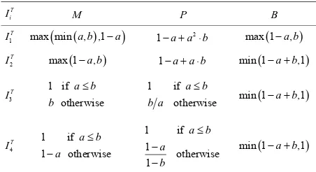
0.1304, i.e., fuzzy sets BTable 6. A
B milar.
for Reichenbach S-implication.
A
T u1 u2 u3 u4 A S A A
,
M 0.35 0.53 0.95 1.0 A 0.820
P 0.23 0.45 0.95 1.0 A 0.886
B 0.0 0.45 0.95 1.0 A 1.0
Table 7. A fo Kleen -Dien S-implication. r e es
A
T u1 u2 u3 u4 A S A A
,
M 0.35 0.45 0.95 1.0 A 0.825
P 0.23 0.45 0.95 1.0 A 0.886
B 0.0 0.45 0.95 1.0 A 1.0
Table 8. A for Lukasiewic S-implication. z
A A
S A A
,
T u1 u2 u3 u4
M 0.35 0.60 0.95 1.0 A 0.809
P 0.23 0.51 0.95 1.0 A 0.882
B 0.0 0.45 0.95 1.0 A 1.0
Let us execute the reasoning mechanism by INAR. The ults sh i bles 9-11 respectively for
diffe ti nd rm
That is, if
res are own n Ta rent implica ons a t-no s.
B is not exactly match with but these are dissimila e r vent can be ned rough inverse approximate reasoning method. The te
not B
r, th fuzzy esol obtai
th
chnique is very new one.
Theorem 7: Let BB be normal and R be interpreted by any implication satisfying Equation (7). Then AUN NOWN for any t-norm T.
Proof:
K
A u
,
sup B A B A B
v V
B A
T v v u v
v
min ,
sup
1, sup
since 1 0.
B A B
B v V
A B
u
v u u v
v
u v
Hence,
We pr eichenbach S-implication
and
v V
UNKNOWN
A .
ove the theorem for R
min
T only, but the above theorem can be proved for any other implications and any other t-norms in the similar way.
Example 4: In Example 2, if we take
1 2 3 4
uation (4) then either by SIAR or by INAR we get B S
MALL 1.0 0.65 0.15 0.0
B v v v v in
Eq
1 1.0 2 1.0 3 1.0 4 UNKNOWN
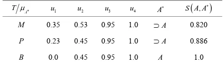
[image:7.595.307.537.103.171.2] [image:7.595.310.537.201.268.2] [image:7.595.308.538.298.372.2]Table 9. Another A for Reichenbach S-implication.
A
T u1 u2 u3 u4 A S A A
,
M 0.15 0.53 0.95 1.0 A 0.9144
P 0.11 0.45 0.95 1.0 A 0.9458
[image:8.595.56.285.199.269.2]B 0.0 0.45 0.95 1.0 A 1.0
Table 10. Another A for eene-Dienes -implication. Kl S
A
T u1 u2 u3 u4 A
,
S A A
M 0.15 0.45 0.95 1.0 A 0.9250
P 0.11 0.45 0.95 1.0 A 0.9458
[image:8.595.58.286.296.367.2]B 0.0 0.45 0.95 1.0 A 1.0
Table 11. Another A for Lukasiewicz S-implication.
A
T u1 u2 u3 u4 A
,
S A A
M 0.15 0.60 0.95 1.0 A 0.8939
P 0.11 0.45 0.95 1.0 A 0.9458
B 0.0 0.45 0.95 1.0 A 1.0
all of th case
Theorem L norm l an
interpreted plica on
Equation (7). Then e s.
8: et Bnot B be a d R be by Rescher-Gaines R-im ti satisfying
AA for an nor
Proof:
Example 5: For the data given in Example 2, applying
INAR for Recher-Gaines R-implication combined with any t-norm , we get the fuzzy resolvent
y t- m T.
A
0,1
1 ,
sup
1 ,
notA b
T b I
not not
not not ,
1 , 1 ,0
sup sup
max sup 1 ,0 sup 1 .
A A
A A
u b u b
A
u b u b
u
u b
T b T b
b b
max
u
T A as
1 2 3
0.0 0.35 0.85 1.0 4
A u u u
bset of A and S A A
,
0.929. It rem 8.u which is a
su establishes Theo-
Observation: In Example 2, for another
1 2 3 4
0.0 0.1225 0.7225 1.0 not
B v v v v B, we
also get the fuzzy resolvent
1 2 3 4
0.0 0.12 0.72 1.0
A u u u u
th Rescher-Ga
r, considering other R-implications, except, Luka-
si sol-
vent
A w h e n w e
apply INAR wi ines R-implication.
Howeve
ewicz R-implication we cannot get such a fuzzy re A which is a subset of A for the same
vent obtained is significant.
We are now going to aplpply another m
input data, although the fuzzy resol
[image:8.595.67.279.436.547.2]ethod SIAR [13] to obtain fuzzy resolvent for the scheme given in Table 1. Let us consider another classical logic equi- valence
a b b a b a (8) The classical logic equivalence (8) can be extended in fuzzy logic with implication and negation function. Then we transform the rule in Table 1 into its equivalent form “p1: If Y is notB then X is A” over the domain
of
0,1V U. A f ule m be def ned by means of a
fo a fu Ca
th
uzzy r r defining
ay zzy
i rtesi
conjunction an product rather
an in terms of a multivalued logic implication [13,22]. Therefore, the rule in p1 is transformed into fuzzy
relation R as
,
1
,
,R v u T B v A u
(9)
where T is a t-norm describing a fuzzy conjunction. Now we can apply our method SIAR described in [13].
Th :
SIAR:
Step 1. Translate given premise a e algorithm is as follows
ALGORITHM-FR
1
p nd compute
not ,
R B A
2
by Equation (9).
Step . Compute similarity measure S
not ,B B
using some suitable definition .Step 3. Modify R
not B,A
with S
not ,B B
to lationobtain the modified conditional re R
not ,B A B
usStep 4. U eration on ing Scheme C in (3).
se sup-projection op
not ,B A B
R to obtain A as
t ,
A B A B
We shall illustrate the method applied su
no , .
R v
v u (10)
here by some
Ex L ample 2. For
completely dissi th or different t-norms the shapes of fuzzy resolvent
sup u
itable examples.
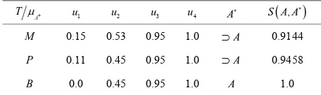
ample 6: et us consider the data in Ex
milar B* wi B and f
T , A
ub in
, when we apply SIAR. The s seq results are U
uent
are studied here
shown in Table 12. In each case, it turns out exacltly the fuzzy set A which corresponds
`
LARGE
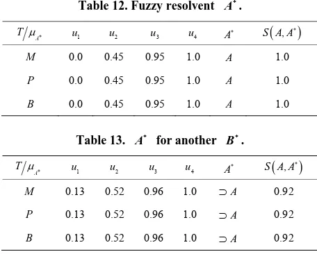
.Example 7: Consider the data in Example 2 where B is not completely dissimilar with B, but dissimilarity
ceeds certain threshold. Then, a lying IAR we ob- serve the shapes of
ex pp S
A and compare it with given A for different t-norms, which is shown in Table 13.
Since S A A
,
0.9255, i.e., A is al st similar tomo A, it establishes fuzzy resolution in reasoning. In the above methods, we apllied INAR or SIAR when the disjunctive knoledge can be transformed into fuzzy implication. However, it may not always be the cas . Moreover, when the expert knowledge is in co
e mplex fo isjunction it is diffi ap
w n deal
with complex premises.
rm of d cult to ply INAR or SIAR.
Table 12. Fuzzy resolvent A.
A
T u1 u2 u3 u4 A S A A
,
M 0.0 0.45 0.95 1.0 A 1.0
P 0.0 0.45 0.95 1.0 A 1.0
B 0.0 0.45 0.95 1.0 A 1.0
Table 13. A for another B.
A
T u1 u2 u3 u4 A S
,
A A
M 0.13 0.52 0.96 1.0 A 0.92
P 0.13 0.52 0.96 1.0 A 0.92
B 0.13 0.52 0.96 1.0 A 0.92
5. Fuzzy Re
i
In t sec w al en he scheme
Table 1. Let
solution w th Complex Clauses
his tion, e sh l ext d t given in
X, Y and Z
cal k
be three linguistic
bles k o n U, V nd W ec-
tively. We e a of an inex on-
clusion “ ” f typi nowledge (premises) “ ” , varia- that ta e valu
id rom
es from the d mai a resp cons er th deriv tion act c
r two p
4 and “q” acording to the scheme given in Table 1 where A ’s, B ’s and C ’s are approximations of
d c ip
positional rule inference. We have found th
basis of the observation
co y to mod
ules so th e shortfall n be re
y g e-defined threshold value,
w
possibly inexact concepts by fuzzy sets over U, V and W respectively.
In 1993, Raha and Ray [12] applied Zadeh’s [23] concept of approximate reasoning with the application of possibility theory to model a deductive process “Genera- lised Disjunctive Syllogism”. They used projection prin- ciple an onjunction princ le to deduce fuzzy resolvent. However, the method could not reduce the shortfall of Zadeh’s Com
e shortfalls in [12] as follows:
1) Let fuzzy resolvent be R for B not B in the scheme given in Table 14, by the method of Raha and Ray [12]. The fuzzy resolvent also be same R for taking B as either B notB or B not .B
2) If we interchange B and B the same fuzzy re- solvent R will be produced.
Therefore, firing a rule on the
uld be harmful. So, it is necessar ify the relation generated by the two given premises, with the similarity measure of two fuzzy sets involved in the
disjunctive form of r at th ca
moved. If a pair of fuzzy sets involved having dis- similarit reater than certain pr
e get our expected fuzzy resolvent using some de- ductive reasoning. Hence, we investigate another method which is described in the following algorithm.
ALGORITHM-FRCEP:
Step 1. Translate the premise p into fuzzy relation
1
R U V
Table 14. Generalised fuzzy resolution—extended form.
p : X is A or Y is B
q : Y is B or Z is C
r : X is A or Z is C
as
1 , min ,1 ;
R u v A u B v
Step 2. Translate p into fuzzy rel
asthe remise
q
ation
2
R VW
2 , min ,
R v w B v w
C
;Step 3. Take cylindrical extension of R1 U Vin
on ,U V W say R1, defined by
1
1 U V W R , , , ;
R
u v u v wStep 4. Take cylindrical extensi ofon R2 in V W
on ,U V W say R2, defined by
2
2 U V W R , , ,
R
v w u v w ; Step 5. Construct RR1∩R2, where ∩ deany perator;
notes fuzzy conjunction
Step 6. Compute o
,
S notB B and, say, ; s Step 7. Modify R with s by Sche C in and, say, R
me (3)
;
Step 8. Obtain R projR on UW defined by
* on sup , , , ;
v
U W R
projR U W
u v w u wStep 9. Obtain A and C by ojecting R eparately
on t
pr s
U and W such tha A proj RU
UsupwR
u w u,
an d
,
. supW W u R
C proj R
u w whe fuzzy re t ,
for
Symbolically, t solven R is obtained by uU, v V and w W ,
, sup , ,
sup
R u w v R u v w
s
1 2 , , , from 3 , ,
sup
, , , , ,
sup
, ,
sup
min ,1 ,
sup
min ,
min ,1 inf ,
min sup ,
, ,
R v
R v
A B
v
B C
A v B
B C
v
A C
u v w
s u v w
1 , 2R R
v
R R
v
s T u v w u v w
u v v w
s T u v
v w
s T u v
v w
s T u w
s T
iff 1 inf vB v supvB v 1.This derivation can be achieved if there is a v0V
is possi- ilar, i.e.,
in
such that and which
dissim
and plication
derivation. We observe two criteria here. Criterion 1: Taking
0 0B v
ble if the fuzzy sets B are si
0 1B v
and B are milar for any im
B notB
min 1, ,
x y y x we get
,
min 1,
,
R u w T A u C w s
;Criterion 2: Taking x y 1 x xy, we get
. C
From above two criteria we observe that when , i.e., when and are com-
herefore, , if
,
1
,
R u w s T A u w s
not ,
0sS B B pletely similar fuzzy resolvent coul
B
UNKN
hing
B
. T ever
OWN
R U W
d be anyt . How s is
st dissimilar close to unity, i.e., if
we
B and B are almo have R is close to
A , C
,
U W
T u w u w
which, after re-translation, gives “If X is A or Z is that a smal ng
C”. Again, we observe l cha e in B pro- duces a small change in fuzzy resolvent—which ensures our method is resonable one.
e another method zzy
re ex set of clauses. ved
that, to obtain a fuzzy resolvent from two clauses containi
the sam
er
e fidence of which is measured
by the dissimilarity measure of the c mplementary literals. However, in the case of almost complementary
bu m
measure of complementary lit
Let us consider a scheme given in Table 15 where
Let us now investigat to find a fu
solvent from a compl It is obser
ng a pair of complementary literals defined over e domain. If the dissimilarity measure of the complementary lit als is unity then we get the resolvent by the disjunction of remaining literals and subsequent removal of the complementary literals. The keyword of the fuzzy resolvent is any one of the complementary literals, th degree of con
o
literals for which dissimilarity value does not attain unity, t exceeds a certain pre-defined threshold, we odify the remaining literals with the measure of dissimilarity in such a way that dissimilarity
[image:10.595.312.538.102.177.2]erals tends to unity and we obtain the resolvent by taking the disjunction of modified literals removing the complementary literals. If the dissimilarity measure of a pair of literals is either zero or close to zero, we cannot obtain a fuzzy resolvent. In this way, we can proceed for a method to find out the derivation of the empty clause and establish the refutation method for the proof of a theorem. The degree of confidence of the empty clause is measured by the degree of confidence of keyword that generated the empty clause and, thus, a sort of com- pleteness of fuzzy resolution principle is established.
Table 15. Generalised fuzzy resolution—another extension.
1
C : X1 is A1 or X2 is A2 or or Xm is Am; 2
C : Y1 is B1 or Y2 is B2 or or Yn is Bn ;
1, 2
R C C : X1 is A1 or or Xm is Am
or Y1 is B1 or or Yn is Bn
variables Xi
i1, 2, , m
and the respective fuzzysubsets A ii
1, 2, , m
are defined on universe
1, 2, ,
i
U i m repectively; variables Yj ( = 1, 2, , )j n and the respective fuzzy subsets Bj 1, 2, ,
j n
aredefined on universe Vj 1, 2, ,
j n
repectively.
A Bk, l
is almost complementary over the same uni- verse Uk
Vl
with the degree of confidence of key-word Ak is cd A
k 1 S A B
k, l
and the rre- cosponding A Bi, j are defined over U Vi, j respectively.
To show the method we set up an algorithm FRAE as follows
ALGO E:
Step h m o e
:
RITHM-FRA
1. C eck the do ain f pair of lit rals
A Bi, j
, ,i j
from clauses
2. If t p e same o
1 and C2
C ;
s in
Step he air remain th d main, say,
k l
U V then m asur the issim larite e d i y f o
A Bk, l
; rwise, there is no fuzzy resolvent;Dissimilarity of Othe
Step 3.
A Bk, l
, i.e., D A B
k, l
iscomputed by 1S A B
,
If
;
k l
Step 4. D A B
k, l
is very very high, i.e.,
k, l
,D A B is pre-defined th o the next step and say, k
reshold then go t
A is ise, there is
resolvent;
Step y Bi either by
keyword; Otherw
5. Modif no fuzzy
min 1, ,
j j k l
B B D A B
or by B j 1
1 Bj
S A
k, l
;Step 6. Fuzzy resolvent is B
1, 2
1 m 1 nR C C A AB B
and
2
cd
R C C1, cd Ak whic ih s measured as cd A
k D A B
k, l
;Step 7. Repeat the process until empty clause, e co
with th nfidence cd0, is derive ore than ses.
Hence, we prove the (u ility of by
the de
d for m two clau n)satisfiab a theorem empty clau
ses.
W trate the models presented
paper. Let us consider variables that range over
fin ated by variables ranging
over such sets.
Example 8: Consider the premises
duction of se from a set of fuzzy clau-
6. Artificial Examples
e consider examples to illus in this