A Particle Swarm Optimization Algorithm for a 2-D
Irregular Strip Packing Problem
Mohamed A. Shalaby, Mohamed Kashkoush
Mechanical Design and Production Department, Faculty of Engineering, Cairo University, Giza, Egypt Email: [email protected]
Received December 12, 2012; revised January 15, 2013; accepted January 28,2013
ABSTRACT
Two-Dimensional Irregular Strip Packing Problem is a classical cutting/packing problem. The problem is to assign, a set of 2-D irregular-shaped items to a rectangular sheet. The width of the sheet is fixed, while its length is extendable and has to be minimized. A sequence-based approach is developed and tested. The approach involves two phases; opti- mization phase and placement phase. The optimization phase searches for the packing sequence that would lead to an optimal (or best) solution when translated to an actual pattern through the placement phase. A Particle Swarm Optimi- zation algorithm is applied in this optimization phase. Regarding the placement phase, a combined algorithm based on traditional placement methods is developed. Competitive results are obtained, where the best solutions are found to be better than, or at least equal to, the best known solutions for 10 out of 31 benchmark data sets. A Statistical Design of Experiments and a random generator of test problems are also used to characterize the performance of the entire algo-rithm.
Keywords: Cutting and Packing; Irregular Strip Packing; Nesting; Placement Procedures; Particle Swarm Optimization
1. Introduction
The problem of packing or cutting out shapes with minimal waste is a classical problem that exists in many industrial fields. Common applications are found in sheet metal, leather, furniture, shipbuilding, and textile Indus- tries. Cutting stock, trim loss, bin packing, strip packing, pallet loading, nesting, and knapsack problems, are all related names for cutting and packing problems. The first general classification for cutting and packing problems is introduced in Dychkoff [1]. Dychkoff developed a spe- cial classification for cutting and packing problems in which he called it a typology. Recently, an improved typology was developed by Wäscher [2], which is par- tially based on Dyckhoff’s original one, but it adopts new categorization criteria.
The scope of this research is the two-dimensional Ir- regular Strip Packing Problem which is classified as an Open Dimension Problem (ODP), according to Wäscher’s improved typology. The problem is to assign (cut or pack), a set of two-dimensional irregular-shaped items to a rectangular object (sheet for cutting or container for packing). The width of the object is fixed, while its length is extendable and has to be minimized. A typical application for this problem is found in the textile Indus- try under the name “Marker-Making”. Another popular name is “Nesting” which has been, and still, used by
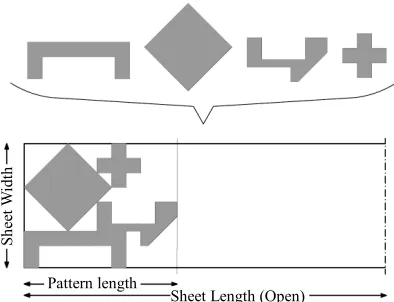
many authors for the Irregular Strip Packing Problems, and even for other irregular cutting and packing prob- lems in general. The problem is schematically demon- strated in Figure 1, where the best arrangement for the
given items into the strip to minimize the pattern length is sought.
The 2-D rectangular packing problem has been shown by Fowler et al. [3] to be NP-complete. As the irregular case is more complex, hence it could also be considered as NP-complete, and as a result they are practically tack- led through heuristic approaches. Two main heuristic approaches are applied; sequence-based approach and direct approach. The first approach utilizes an optimiza- tion technique to find the packing sequence of items that would lead to the best possible pattern when employed under a certain placement method (Babu and Babu [4], Fischer and Dagli [5], Takahara et al. [6], and Burke et al. [7]). While the second approach heuristically builds an initial pattern that may not be a feasible one, and an op- timization technique is directly applied to the items posi- tions seeking the best possible feasible pattern (Bennell and Dowsland [8], Gomes and Oliveira [9], Immamichi et al. [10], and Umetani et al. [11]).
Sh
ee
t W
idt
h
[image:2.595.73.270.86.237.2]Sheet Length (Open) Pattern length
Figure 1. A schematic illustration for the 2-D irregular strip packing problem.
and Daniels [12] and Fischetti and Luzzi [13], Constraint Logic Programming (CLP) approach followed by Carra- villa et al. [14], and dynamic sequence-based approach followed by Oliveira et al. [15], and Bennell and Song [16].
Developing a geometrical technique for handling the graphical aspects of irregular shapes is used to be the main obstacle among extending the research in this problem, compared to the regular cutting and packing one. Three geometry handling techniques are widely used in the literature. Pixel or Raster Method is an ap- proximate method that is employed by Jain and Gea [17], Babu and Babu [4], and Fischer and Dagli [5]. Direct trigonometry techniques are used by Hifi and M’Hallah [18], Takahara et al. [6], and Burke et al. [7]. A more sophisticated technique is the no-fit polygon which is applied by Oliveira et al. [15], Bennell and Song [16], and Imamichi et al. [10].
Many authors used to incorporate meta-heuristic search techniques in their solution algorithms. Three main meta-heuristics are commonly used with irregular cutting and packing problems, they are; Genetic Algo- rithm (Jakobs [19], Hifi and M’Hallah [18], and Hu-yao and Yuan-jun [20]), Simulated Annealing (Oliveira and Ferreira [21], Han and Na [22], Heckmann and Lengauer [23], and Gomes and Oliveira [9]), and Tabu Search (Blazewicz et al. [24], Bennell and Dowsland [8], and Burke et al. [7]).
From the above review, much interest could be noticed in the Irregular Strip Packing Problem for the last few years. This could be attributed to two main reasons; firstly, until now, no optimal solution could be found for a real-sized problem, a very small improvement in a given arrangement in a cutting or packing operation could save a considerably large amount of money. Sec- ondly, is the significant increase in the capabilities of modern computational engines, which made it available to apply techniques that would be impractical to apply 15
years ago. Several heuristic and meta-heuristic optimiza- tion techniques have been applied and investigated with the problem. Particle Swarm Optimization (PSO) algo- rithm, originally introduced by Kennedy and Eberhart [25], is a lately developed stochastic optimization tech- nique that has proved good performance in various opti- mization fields, but has not been applied to a Strip Pack- ing Problem or any cutting or packing problem. This research investigates the performance of PSO to find a competitive (or even better) performance to the existing approaches.
2. Proposed Solution Approach
The solution approach proposed in this paper, which is given the name “SwarmNest”, is a sequence-based ap- proach that consists of two phases; optimization phase and placement phase. SwarmNest assumes only hole-free polygons that are allowed to rotate by increments of 90˚.
For the optimization phase, a Particle Swarm Optimi- zation (PSO) algorithm is employed to search for the optimal packing sequence. Up to our knowledge, this is the first time Particle Swarm is utilized in tackling an irregular packing problem. A proposed Local Search routine is also used to enhance the algorithm perform- ance. As to the placement phase, a combined placement algorithm is developed and employs two different ge- ometry handling techniques; pixel method and direct trigonometry. The algorithm involves two stages; the first is an initial placement stage that applies a pixel- based placement procedure, which alternatively could be a D-function-based one. The second is a refinement placement stage that incorporates a heuristic compaction routine. A general flowchart for the entire approach (SwarmNest) is shown in Figure 2.
The remaining of this paper is organized as follows. In the next Section, the combined placement algorithm along with the employed geometry handling techniques is explained. The proposed Particle Swarm Optimization algorithm is described in Section 4. Then, the experi- mental results of the entire approach (SwarmNest) are presented in Section 5. SwarmNest performance is then characterized in Section 5. Finally, the summary and main conclusions are presented in Section 6.
3. Combined Placement Algorithm
Items geometry Particle Swarm paramete Placement algorithm param
rs eters
Generate initial packing sequences
Run the combined placement algorithm
Run Particle Swarm Optimization algorithm
Termination criterion met
Best solution pattern Start
[image:3.595.84.258.79.341.2]End Yes No
Figure 2. A general flowchart for the entire approach (SwarmNest).
raster) method, and direct trigonometry. Pixel method is employed under a pixel-based placement procedure dur- ing the initial placement stage; while direct trigonometry is applied through a heuristic compaction routine during the refinement placement stage.
3.1. Stage I: Initial Placement
3.1.1. Pixel Method
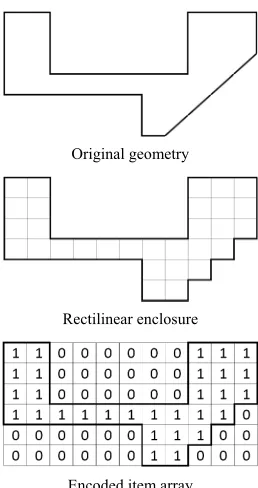
Pixel method is an approximate geometry handling tech- nique. The geometry of an item through this method is first approximated by a set of square cells that form a rectilinear enclosure. Such an approximated form is then encoded by a 2-D array (item array). An item array in- volves two types of cells: interior and exterior cells. An interior cell is the one corresponding to one of the recti- linear enclosure cells, while other remaining cells within the item array are exterior cells. Figure 3 illustrates the
idea through the simplest encoding scheme; the binary encoding scheme used by Oliveira and Ferreira [21].
In the same manner, the placement sheet is encoded by a 2-D array (sheet array). This array also involves two types of cells; occupied and unoccupied cells. Occupied cells are those cells utilized via former placement opera- tions, while unoccupied cells are the remaining free cells. Assigning a certain location inside the sheet to a given item is done by adding the corresponding item array, to the sheet array at that place. Hence, for a feasible place- ment (overlap-free placement), any of the interior cells of the item array should not be added to an occupied cell
Original geometry
Rectilinear enclosure
[image:3.595.358.487.82.326.2]Encoded item array
Figure 3. Geometry encoding through binary encoding scheme (Oliveira and Ferreira (1993)).
within the sheet array.
3.1.2. Initial Placement Algorithm
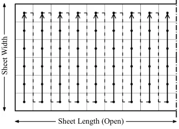
The strategy by which the algorithm works is a scanning strategy. Each time a new item is required to be placed or packed, the sheet is scanned through a predefined path for the first feasible available positioning for that item. The path by which the sheet array is scanned is exhibited in Figure 4.
Accordingly, the scanning is carried out along the sheet length direction from left to right, where each col- umn is scanned from bottom to top; usually called bot- tom-left placement policy. The default starting position is the sheet origin, while in order to reduce the scanning time, an item starts its scanning path from the farthest position a smaller item, or even the same item, has reached. A smaller item is the one that has a smaller area, length, and width than the item being placed. In this way many potentially infeasible positions are neglected.
During the placement procedure, feasibility check, at each of the scanned position is carried out for each of the allowed orientations (0˚, 90˚, 180˚, and/or 270˚). The selected orientation is the one with the highest contacting condition; contact with other already placed items and with the sheet borders.
3.2. Stage II: Refinement Placement
3.2.1. Direct Trigonometry Method (D-Function)
Sheet Length (Open)
Sh
ee
t W
idt
[image:4.595.345.503.86.179.2]h
Figure 4. Proposed scanning path.
by their actual geometries (hole-free polygons), where the direct trigonometry method described by Bennell and Oliveira [26] is employed as a geometry handling tech- nique. Accordingly, an overlap between any two items is detected through three consecutive levels of trigonomet- ric tests. The core calculations are carried out through the third level. This level detects intersection between any two lines that have an overlap potential (according to the former levels). A mathematical function known as D- function is employed through this level. It was first pro- posed by Konopasek [27], and the D-function is given by the following expression:
ABP A B A P
A B
A P
D X X Y Y Y Y X X
0
D
0
D
0
D
0
(1)
Upon calculating the D-function value for a point P and an oriented edge AB, the relative position of P with respect to AB, as well the extension of AB in both directions (an infinite line), could be defined according to the sign of DABP. If ABP , then P is on the left side of AB and its extensions. If ABP , then P is on the right side of AB and its extension. While If ABP , then P lies on AB or its extension. Figure 5 presents the case where P is on the left side of AB DABP .
3.2.2. Refinement Placement Algorithm
The second stage of the combined placement algorithm applies a heuristic compaction routine on the pattern ob- tained from the first stage. A similar routine to the pro- posed one is found in Hopper [28] as “iteration routine”. Another one is introduced by Jakobs [19] as “shrinking algorithm”. Both authors primarily employ a rectangular enclosure representation for the items.
[image:4.595.81.264.90.222.2]Through the proposed routine, the compaction process is carried out on a number of successive identical passes. A compaction pass sequentially considers the items one by one. Each of the considered items is tried for compac- tion in eight directions; leftward firstly then upward, downward, up-left, and down-left. Compacting an item in a given direction is performed by incremental transla- tional movements carried out in that direction.
Figure 5. The case at which the value of DABP is greater than
zero.
After each movement, the item’s new position is checked for being a feasible one (no overlaps). If the new position is feasible, then it is being approved and the compaction process is continued in that direction, other- wise the item retrieves its last feasible position before continuing to the next compaction direction. The routine is performed via more than one pass so as to utilize the probable in between gaps, resulted after each pass.
4. Particle Swarm Optimization
Particle swarm optimization (PSO) is a population-based stochastic optimization technique devised to model the social behavior of animals, birds, or insects. It was origi- nally developed by Kennedy and Eberhart [25]. PSO has been successfully applied to several classical optimiza- tion problems such as; scheduling, traveling salesman, network deployment, task assignment, and neural net- work training problems (Blum and Merkle [29]). PSO is used here during the optimization phase of SwarmNest to search for a better placement sequence, where the feasi- bility and value yielded by any sequence is assessed by applying the combined placement algorithm.
4.1. Basics of Continuous Particle Swarm Optimization
In PSO, individual particles represent possible solutions, which spread through the problem search space looking for an optimal, or even a good enough solution, and each particle transmits its current state to other particles in the population. In an evolutionary manner, the position of each particle is updated according to its current position, the particle’s best position so far (personal best position), and the global best position ever found by the whole population. As the search continues, the whole swarm is supposed to be directed more and more towards the posi- tion corresponding to the global best solution for the whole population. The textbook of Blum and Merkle [29] is a good introduction for PSO.
the position vector represent the set of continuous deci- sion variables. Then the fitness (objective value) of each particle is evaluated as a function of its current position so as to find the particle of the highest fitness. The first iteration is then started by updating both the position and the velocity vectors of the entire population according to Equations (2) and (3).
1 1
i i i
n n n
x x v (2)
2 2
g i n n
c r p x
,
r r
1 1 1
i i i i
n n n n
v v c r p x (3)
where:
i: Refers to the ith particle of the swarm
n, n + 1: Denote iterations, n being the current itera- tion.
1 2: Pseudo-random numbers in the interval [0, 1],
generated for each variable within each particle at each iteration
x: Position vector whose elements are decision vari- ables 1, , ,2 m
x x x , where m is the number of decision variables.
v: Velocity vector. i
p : Personal best position vector found by particle
initially i
o
i x .
g p
,
c c
: Global best position vector through the whole swarm.
1 2: Adjustable optimization parameters used to
control the swarm’s behavior, both values are kept fixed for the entire algorithm.
New fitness values are evaluated at the updated parti- cle’s positions, and the best position found so far by each particle, as well as the global best position, are updated. The procedure is then continued until a predefined ter- mination criterion is met. An additional adjustment can be applied to Equation (3), whereby velocity is updated, by inserting what is known as inertia reduction weight
, hence the velocity equation is to be written as shown in Equation (4):
c r2 2
pngxni
1 1 1
i i i i
n n n n
v v c r p x (4)
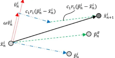
The schematic vector diagram in Figure 6 illustrates
the updating process of a position vector according to Equations (2) and (4).
4.2. Proposed PSO Algorithm
[image:5.595.328.521.87.185.2]Based on the approach followed by Tasgetiren et al. [30] in tackling the flow shop scheduling problem, our pro- posed PSO algorithm for finding the optimal packing sequence is a continuous one that employs a proposed criterion in extracting the actual solutions. Through the proposed algorithm, the position of a particle, denotes a packing sequence, is represented by a vector with the same length of the total number of items. The value of
Figure 6. A schematic vector diagram for updating position vector i.
n x
each element in the position vector always imply an item number, thus it initially takes a positive integer number from 1 to total number of items. Thus, the initial position vectors represent a set of feasible packing sequences. Hence, the velocity value of a given particle is equivalent to a difference between some two items numbers. Veloc- ity values are initially set to zero. The initial population is made up of two sets of sequences. The first set in- volves the result of applying 10 heuristic ordering rules (e.g. by area, by length, and by width), while the other set is completely randomly generated sequences.
The velocity vectors are updated using Equation (4) that incorporates inertia reduction parameter
, but additionally a decrement factor
is multiplied by
during each iteration as in Tasgetiren et al. [30]. This would results in a gradual increase in the inertia reduction with consecutive iterations; hence, a premature convergence is to be avoided in early iterations, while an intensive search behavior could be realized in later ones. A minimum value for
is preserved to prevent the complete elimination of the inertia term in the velocity equation.Moreover, the applied velocity limits are always set to be half the total number of items in both directions (posi- tive and negative); this would force the velocity and po- sition values to be always in magnitude of the initial po- sition values that signify items numbers. A proposed cri-terion is applied for obtaining the actual discrete se- quence from a given continuous position vector. Each element i in the position vector contains a real value (− or +). The order of the ith element, when all elements are ascendingly ordered, becomes the ith element in the ac- tual sequence (see Figure 7).
In addition, an item number is originally assigned based on its area, relative to other larger or smaller items, that is, the number 1 is given to the item with the small- est area and so on. Thus, the value taken by each position element implies a physical meaning. A pseudocode for the proposed PSO is outlined below.
Input c c1, ,2 , min,Np,vmin,vmax,Tmax //parameters 1
g
Set //initially set global best particle to be
Variable: 1 2 3 4 5 6
Pos. vector: 1.80 −0.99 3.01 −0.72 −1.20 2.15
[image:6.595.309.539.85.325.2]
Act. seq.: 4 2 6 3 1 5
Figure 7. Proposed solution extraction criterion.
Fori = 1 to Np //Np is the population size
Initialize x vi, i
xiZ i Evaluate //call the placement
algo-rithm
Set i xi, st
i Z i
p Be
If Z i
Z
gmax tT
0,1 r rand
min ij
v v
min ij
v v
x ij
v v
max ij
v v
ij
g = i //global best particle
End if Nexti
While //Tmax is the maximum no. of
it-erations t = t +1
Fori = 1 to Np
Forj = 1 to Total no. of items
1 0,1 , 2
r rand
ij v
Update //Equation 4 (velocity equation) If ,
Else if ma ,
End if
Update x //Equation 2
Nextj
i i
s Extract x //proposed extraction criterion
iZ i s
EvaluateIf Z i
Best
iSet est
i Z i
i Best
g, B
i i
p x //update
personal best
End if
If Best ,
gi //update global best
End if Next i End While
4.3. Local Search Routine
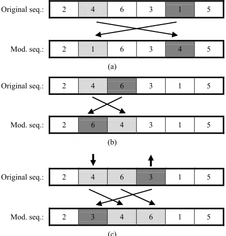
The performance of PSO algorithms are highly improved when local or neighborhood search is integrated to it. The proposed Local Search routine applies three Local Search operations; interchange between two randomly selected items (Figure 8(a)), interchange between a ran-
domly selected item and its consecutive one (Figure 8(b)), and Insertion of a randomly selected item into a
randomly selected place (Figure 8(c)).
An interchange operation is completed if only the items to be interchanged represent different items. Those
Original seq.: 2 4 6 3 1 5
Mod. seq.: 2 1 6 3 4 5
(a)
Original seq.: 2 4 6 3 1 5
Mod. seq.: 2 6 4 3 1 5
(b)
Original seq.: 2 4 6 3 1 5
Mod. seq.: 2 3 4 6 1 5
(c)
Figure 8. Applied local search operations: (a) Interchange between two randomly selected elements; (b) Interchange between a randomly selected element and it’s consecutive; (c) Insertion of a randomly selected element to a randomly selected place.
operations are applied during each PSO iteration. The Local Search routine is carried out for both; global best sequence (obtained from
pg ) as well as the personal best sequence of each particle (obtained from
pi ). The entire routine is repeated up to a predefined number of local search iterations.5. Experimental Results
In this section, SwarmNest is benchmarked and charac- terized. Firstly, the results obtained by SwarmNest for 31 benchmark data sets available in the literature are com- pared with the published results. Then, 25 factorial de- sign of experiments is conducted to characterize Swarm- Nest performance. Experiments are conducted on a lap- top of 1.5 GB RAM supported by an Intel® Core Duo
processor of 1.66 GHz CPU speed and 2 MB cache size, operated with a Microsoft Windows XP Professional O/S, and algorithms are written in Visual Basic.
5.1. Benchmarking of SwarmNest
[image:6.595.53.294.85.584.2]optimum of 100% utilization. Additional 9 problems (from Poly1a to Poly5b) were also randomly generated and documented for testing purposes. All the data sets in Hopper [28] are collections of hole-free polygons that do not include any internal holes or arcs. Hopper’s data sets were then made available by the EURO Special Interest Group on Cutting and Packing (ESICUP)
(http://paginas.fe.up.pt/~esicup/).
In Burke et al. [7], 10 new data sets (Profile1, ..., Pro- file10) were introduced for benchmarking purposes. Only three data sets are included, and two of which are jigsaw problems (Profile7 and Profile8). Others are not included as they contain holes and/or arcs in the shapes of their items. Furthermore, we extracted a single data set (Grinde) from Hifi and M’Hallah [18].
Seven sets of published results were available for our comparison; the first set is definitely the results obtained by Hopper [28]. Few years later, Gomes and Oliveira [9] introduced the first published results to consider Hop- per’s data sets. They also conducted a comparison be- tween the best ever results published for Hopper’s data sets and the corresponding results obtained by their own algorithms; SAHA and GLSHA. Gomes and Oliveira reported improvements over the best known results for 15 data sets, but they considered only 15 out of the 18 data sets, and did not consider any of the data sets Poly1a to Poly5b. Gomes and Oliveira [9] results and compari- sons were then used as the basis for the subsequent lit- erature comparisons. Such comparisons are reported in Egeblad et al. [31], Bennell and Song [16], Imamichi et al. [10] and Umetani et al. [11]. Also Burke et al. [7] introduced 10 new data sets, in addition to considering almost all Hopper’s data sets in their reported compari- son.
SwarmNest allows Particle Swarm to be used with ei- ther a combined pixel-based, or alternatively, a combined D-function-based placement algorithm. The alternative placement algorithm applies a D-function-based place- ment procedure during its first stage, instead of the pixel-based one described in the second section. Both procedures are conceptually similar to a great extent, in which both adapt the same scanning strategy. The com-bined pixel-based algorithm is the main one, but some data sets would be better tackled with the combined D-function-based algorithm, especially those that are either jigsaw saw or randomly generated data sets. Hence, 14 data sets (Han, Dighe1, Dighe2, Profile7, Profile8, and Poly1a to Poly5b) were solved with the SwarmNest that employs a D-function-based algorithm.
For every data set, SwarmNest is allowed to run for 20 times and maximum time allowed for each run is set to 1 hour. The best results obtained by SwarmNest along with the best results reported by each of the 7 publications are shown in Table 1, in which a typical utilization% meas-
ure (total items area/(sheet width x used sheet length)) is used as a unified efficiency measure. The best ever solu- tion for each problem is recognized with a grey back- ground.
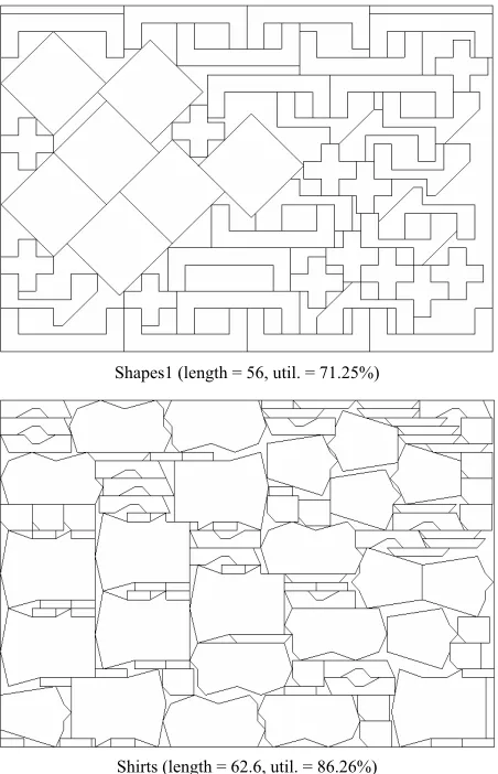
SwarmNest produced better solutions, or at least equal to, the best known solutions for 10 out of the 31 bench- mark data sets. Moreover, the overall average of Swarm- Nest best results over the 31 data sets (78.37%) is better than the average of all the published results (77.47%). A sample from the best solution patterns obtained by SwarmNest is shown in Figure 9.
5.2. Characterization of SwarmNest
In order to characterize the better performance of SwarmNest, a Statistical Design of Experiments ap- proach is adapted. Accordingly, five key factors are de- fined, and two levels are set for each factor, and thus a (25) factorial design with 32 different experiments is used.
The five factors are defined, provided that the value for each factor, excluding the fourth one, is given by the mean value among an entire data set:
Shapes1 (length = 56, util. = 71.25%)
[image:7.595.311.537.355.706.2]Shirts (length = 62.6, util. = 86.26%)
Table 1. Best published results and best results obtained by SwarmNest for the 31 benchmark data sets.
Hopper [28] (2000)
Burke et al. [7] (2006)
Gomes & Oliveira [9] (2006)
Egeblad et al. [31]
(2007)
Bennell & Song [16]
(2010)
Imamichi et al. [10] (2009)
Umetani et al. [11]
(2009) Data set
No. Label
Hopper’s BLF SAHA 2DNest BS ILSQN FITS SwarmNest
1 Blaz1 70.42 79.41 83.60 81.59 81.29 84.25 81.68 80.9
2 Blaz2 63.97 74.5 - - - 74.74
3 Dagli 77.1 83.7 87.15 87.05 87.99 87.40 86.35 83.97
4 Fu 83.82 86.9 90.96 92.03 90.82 90.67 91.23 89.06
5 Jalobs1 74.25 82.6 81.67b 89.07 85.96 86..89 89.09 81.67
6 Jakobs2 68.4 74.8 77.28 81.07 80.40 82.51 80.84 77.2
7 Marques 82.73 86.47 88.14 89.82 88.92 89.03 89.21 86.47
8 Shapes 63.33 67.6 - - - 71.25
9 Shapes0 57.83 61.4 66.50 67.09 65.41 68.44 66.50 65.41
10 Shapes1 62.25 68.3 71.25 73.84 72.55 73.84 73.88 71.25
11 Shirts 79.65 85.7 86.80 b 87.38 89.69 88.78 86.92 86.26
12 Swim 67.42 68.4 74.37 72.49 75.04 75.29 74.54 68.25
13 Trousers 79.12 89.6 89.96 90.46 90.38 89.79 89.40 88.36
14 Albano 84.09 84.6 87.43 87.88 87.88 88.16 87.56 83.36
15 Dighe1 71.01 77.4 100 99.86 100 99.89 99.89 100
16 Dighe2 70.23 79.4 100 99.95 100 99.99 100 100
17 Mao 68.65 79.5 82.54 85.15 84.07 83.44 83.73 78.4
18 Han 68.9 - - - 77.19
19 Poly1aa 69.7 73.2 - - - 73.73
20 Poly2aa 68.1 72.8 - - - 75.33
21 Poly3aa 76.11 76.2 - - - 73.87
22 Poly4aa 72.05 74.6 - - - 73.06
23 Poly5aa 71.57 73.9 - - - 72.86
24 Poly2ba 68.34 75.4 - - - 73.41
25 Poly3ba 73 74.9 - - - 73.43
26 Poly4ba 73.15 74.8 - - - 73.66
27 Poly5ba 72.38 75.8 - - 79.51 - - 72.25
28 Profile7 - 77.1 - - - - - 81.93
29 Profile8 - 75.8 - - - - - 79.98
30 Profile10 - 66.2 - - - - - 63.1
31 Grinde Only Hifi and M’Hallah [18]: 78.6% 78.97
aAll the
1) No. of items (NI): Total no. of items;
2) Size ratio (SR): Length + width of the item, divided
by twice the sheet width;
3) No. of lines (NL): No. of lines or vertices per item
or shape;
4) Coeff. of var. (CV): Standard deviation of the items
areas, divided by mean area;
5) Complexity (C): No. of interior angles which are
greater than 180˚, divided by No. of lines.
The first factor (NI) reflects the dimensionality of a
given problem, as the problem of finding the optimal packing sequence becomes more complicated with larger no. of items. The second factor (SR) expresses the rela-
tive size of an average item size with respect to the size of the placement sheet. The third factor (NL) represents
an aspect of geometrical complexity of a given item. The fourth factor, Coefficient of Variation, (CV) signifies the
extent of variability between different item sizes within the same data set. The last factor (C) is another aspect of
item geometrical complexity; higher complexity factor means higher concavities in an item’s shape, while zero complexity means convex-shaped items.
Two levels, high and low, are selected for each factor. Since generating a data set of random shaped items with an exact value for each factor is very difficult, a range of values is used to specify each factor level. The bench- mark data sets were a good guide for selecting those ranges. The applied range for each factor at each level is shown in Table 2.
Thirty two (25) different experimental runs are con-
[image:9.595.309.536.99.393.2]ducted, where each run consisted of 10 replications, and each replication requires one data set of N Items. Hence, the 320 (32 × 10) data sets are randomly generated and solved by SwarmNest with the combined pixel-compac- tion placement algorithm, as being the main placement algorithm. The sheet width is always set to 60 units and all the items are allowed to rotate by increments of 90˚. Main and interaction effects of the five factors on the response are exhibited in Table 3.
Table 2. Applied range for each factor level.
Low level (−) High level (+) No. Factor
Value Range Value Range
1 No. of items (NI) 20 (10, 30) 50 (40, 60)
2 Size ratio(SR) 0.15 (0.1, 0.2) 0.35 (0.3, 0.4)
3 No. of lines(NL) 4.5 (3, 6) 8.5 (7, 10)
4 Coeff. of var.(CV) 0.45 (0.3, 0.6) 0.95 (0.8, 1.1)
Complexity
(C @ low NL) 0.025 (0, 0.05) 0.125 (0.1, 0.15)
5
Complexity
[image:9.595.60.285.582.734.2](C @ high NL) 0.175 (0.15, 0.2) 0.25 (0.25, 0.3)
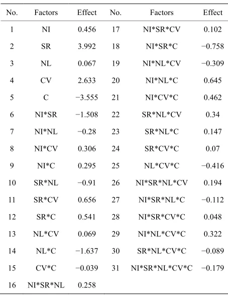
Table 3. Main and interaction effects.
No. Factors Effect No. Factors Effect
1 NI 0.456 17 NI*SR*CV 0.102
2 SR 3.992 18 NI*SR*C −0.758
3 NL 0.067 19 NI*NL*CV −0.309
4 CV 2.633 20 NI*NL*C 0.645
5 C −3.555 21 NI*CV*C 0.462
6 NI*SR −1.508 22 SR*NL*CV 0.34
7 NI*NL −0.28 23 SR*NL*C 0.147
8 NI*CV 0.306 24 SR*CV*C 0.07
9 NI*C 0.295 25 NL*CV*C −0.416
10 SR*NL −0.91 26 NI*SR*NL*CV 0.194
11 SR*CV 0.656 27 NI*SR*NL*C −0.112
12 SR*C 0.541 28 NI*SR*CV*C 0.048
13 NL*CV 0.069 29 NI*NL*CV*C 0.322
14 NL*C −1.637 30 SR*NL*CV*C −0.089
15 CV*C −0.039 31 NI*SR*NL*CV*C −0.179
16 NI*SR*NL 0.258
The response is the sheet utilization, or the algorithm efficiency. A positive sign associated with an effect value means that the response value increases with increasing the corresponding factor value, and vice versa, and the magnitude of the effect represents its relative weight. Statistical package of Minitab 15 is used for calculations and analysis of results.
Clearly, many of the calculated effects appear to be not significant enough, which indicates that SwarmNest performance is of a low sensitivity to a problem attrib- utes. The best performance for SwarmNest is obtained with problems of large relative item sizes, low geometri- cal complexity or irregularity, and high variability be- tween item sizes.
6. Conclusions
In this research, the common industrial problem “2-D Irregular Strip Packing Problem” is addressed, and a heuristic sequence-based approach is developed for solving it. A Particle Swarm Optimization algorithm (PSO) is applied during the optimization phase of the approach, where it is the first time a PSO algorithm is incorporated in solving this problem. The introduced solution approach is given the name “SwarmNest”.
sults were obtained and the best solutions of SwarmNest are found to be better than, or at least equal to, the best known solutions for 10 out of the 31 benchmark data sets.
Furthermore, the performance of SwarmNest is char- acterized through a Statistical Design of Experiments that incorporates a specially designed random problem gen- erator. The results showed that the best performance for SwarmNest is obtained at large item sizes (with respect to the sheet), low geometrical complexity, and high variability between item sizes.
REFERENCES
[1] H. Dyckhoff, “A Typology of Cutting and Packing Prob- lems,” European Journal of Operational Research, Vol. 44, No. 2, 1990, pp. 145-159.
doi:10.1016/0377-2217(90)90350-K
[2] G. Wäscher, H. Haußner, and H. Schumann, “An Im- proved Typology of Cutting and Packing Problems,” European Journal of Operational Research, Vol. 183, No. 3, 2007, pp. 1109-1130. doi:10.1016/j.ejor.2005.12.047 [3] R. J. Fowler, M. S. Paterson and S. L. Tanimoto, “Optimal
Packing and Covering in the Plane Are NP-Complete,” Information Processing Letters, Vol. 12, No. 3, 1981, pp. 133-137. doi:10.1016/0020-0190(81)90111-3
[4] A. R. Babu and N. R. Babu, “A Generic Approach for Nesting of 2-D Parts in 2-D Sheets Using Genetic and Heuristic Algorithms,” Computer-Aided Design, Vol. 33, No. 12, 2001, pp. 879-891.
doi:10.1016/S0010-4485(00)00112-3
[5] A. D. Fischer and C. H. Dagli, “Employing Subgroup Evolution for Irregular-Shape Nesting,” Journal of Intel- ligent Manufacturing, Vol. 15, No. 2, 2004, pp. 187-199.
doi:10.1023/B:JIMS.0000018032.38317.f3
[6] S. Takahara, Y. Kusumoto and S. Miyamoto, “Solution for Textile Nesting Problems Using Adaptive Meta-Heu- ristics and Grouping,” Soft Computing, Vol. 7, No. 3, 2003, pp. 154-159. doi:10.1007/s00500-002-0203-9 [7] E. Burke, R. Hellier, G. Kendall and G. Whitwell, “A
New Bottom-Left-Fill Heuristic Algorithm for the Two Dimensional Irregular Packing Problem,” Operations Re- search, Vol. 54, No. 3, 2006, pp. 587-601.
doi:10.1287/opre.1060.0293
[8] J. A. Bennell and K. A. Dowsland, “Hybridising Tabu Search with Optimisation Techniques for Irregular Stock Cutting,” Management Science, Vol. 47, No. 8, 2001, pp. 1160-1172. doi:10.1287/mnsc.47.8.1160.10230
[9] A. M. Gomes and J. F. Oliveira, “Solving Irregular Strip Packing Problems by Hybridising Simulated Annealing and Linear Programming,” European Journal of Opera- tional Research, Vol. 171, No. 3, 2006, pp. 811-829.
doi:10.1016/j.ejor.2004.09.008
[10] T. Imamichi, M. Yagiura and H. Nagamochi, “An Iterated Local Search Algorithm Based on Nonlinear Program- ming for the Irregular Strip Packing Problem,” Discrete Optimization, Vol. 6, No. 4, 2009, pp. 345-361.
doi:10.1016/j.disopt.2009.04.002
[11] S. Umetani, M. Yagiura, S. Imahori, T. Imamichi, K. Nonobe and T. Ibaraki, “Solving the Irregular Strip Pack- ing Problem Via Guided Local Search for Overlap Mini- mization,” International Transactions in Operations Re- search, Vol. 16, No. 6, 2009, pp. 661-683.
doi:10.1111/j.1475-3995.2009.00707.x
[12] R. B. Grinde and K. Daniels, “Solving an Apparel Trim Placement Problem Using a Maximum Cover Problem Approach,” IIE Transactions, Vol. 31, No. 8, 1999, pp. 763-769. doi:10.1080/07408179908969875
[13] M. Fischetti and I. Luzzi, “Mixed-Integer Programming Models for the Nesting Problem,” Journal of Heuristic, Vol. 15, No. 3, 2009, pp. 201-226.
doi:10.1007/s10732-008-9088-9
[14] M. A. Carravilla, C. Ribeiro and J. F. Oliveira, “Solving Nesting Problems with Non-Convex Polygons by Con- straint Logic Programming,” International Transactions in Operational Research, Vol. 10, No. 6, 2003, pp. 651- 663. doi:10.1111/1475-3995.00434
[15] J. F. Oliveira, A. M. Gomes and J. S. Ferreira, “TOPOS— A New Constructive Algorithm for Nesting Problems,” OR-Spektrum, Vol. 22, No. 2, 2000, pp. 263-284.
doi:10.1007/s002910050105
[16] J. A. Bennell and X. Song, “A Beam Search Implementa-tion for the Irregular Shape Packing Problem,” Journal of Heuristic, Vol. 16, No. 2, 2010, pp. 167-188.
doi:10.1007/s10732-008-9095-x
[17] S. Jain and H. C. Gea, “Two-Dimensional Packing Prob- lems Using Genetic Algorithms,” Engineering with Com- puters, Vol. 14, No. 3, 1998, pp. 206-213.
doi:10.1007/BF01215974
[18] M. Hifi and R. M’Hallah, “A Hybrid Algorithm for the Two-Dimensional Layout Problem: The Cases of Regular and Irregular Shapes,” International Transactions in Op-erational Research, Vol. 10, No. 3, 2003, pp. 195-216.
doi:10.1111/1475-3995.00404
[19] S. Jakobs, “On Genetic Algorithms for the Packing of Polygons,” European Journal of Operational Research, Vol. 88, No. 1, 1996, pp. 165-181.
doi:10.1016/0377-2217(94)00166-9
[20] H.-Y. Liu and Y.-J. He, “Algorithm for 2D Irregular- Shaped Nesting Problem Based on the NFP Algorithm and Lowest-Gravity-Center Principle,” Journal of Zheji- ang University, Science A, Vol. 7, No. 4, 2006, pp. 570- 576. doi:10.1631/jzus.2006.A0570
[21] J. F. Oliveira and J. S. Ferreira, “Algorithms for Nesting Problems,” In: R. V. V. Vidal, Ed., Applied Simulated Annealing, Lecture Notes in Economics and Mathemati- cal Systems, Vol. 396, Springer-Verlag, Berlin, 1993, pp. 255-274.
[22] G. C. Han and S. J. Na, “Two-Stage Approach for Nest-ing in Two-Dimensional CuttNest-ing Problems UsNest-ing Neural Network and Simulated Annealing,” Proceedings of the Institute of Mechanical Engineers, Part B, Journal of En- gineering Manufacture, Vol. 210, No. B6, 1996, pp. 509- 519.
Matching Upper and Lower Bounds on Textile Nesting Problems,” European Journal of Operational Research, Vol. 108, No. 3, 1998, pp. 473-489.
doi:10.1016/S0377-2217(97)00049-0
[24] J. Blazewicz, P. Hawryluk and R. Walkowiak, “Using a Tabu Search Approach for Solving the Two-Dimensional Irregular Cutting Problem,” Annals of Operations Re- search, Vol. 41, No. 4, 1993, pp. 313-325.
doi:10.1007/BF02022998
[25] J. Kennedy and R. C. Eberhart, “Particle Swarm Optimi- zation,” Proceedings of IEEE International Conference on Neural Networks,Piscataway, 27 November-1 Decem- ber 1995, pp. 1942-1948.
doi:10.1109/ICNN.1995.488968
[26] J. A. Bennell and J. F. Oliveira, “The Geometry of Nest- ing Problems: A Tutorial,” European Journal of Opera- tional Research, Vol. 184, No. 2, 2008, pp. 397-415. doi:10.1016/j.ejor.2006.11.038
[27] M. Konopasek, “Mathematical Treatments of Some Ap- parel Marking and Cutting Problems,” US Department of
Commerce, Washington DC, 1981.
[28] E. Hopper, “Two-Dimensional Packing Utilising Evolu- tionary Algorithms and Other Meta Heuristic Methods,” Ph.D. Thesis, Cardiff University, Cardiff, 2000.
[29] C. Blum and D. Merkle, “Swarm Intelligence: Introduc- tion and Applications,” Springer-Verlag, Berlin, 2008. doi:10.1007/978-3-540-74089-6
[30] M. F. Tasgetiren, Y. C. Liang, M. Sevkli and G. Gency- ilmaz, “Particle Swarm Optimization Algorithm for Make- span and Maximum Lateness Minimization in Permuta- tion Flowshop Sequencing Problem,” Proceedings of the Fourth International Symposium on Intelligent Manufac- turing Systems, Sakarya, 6-8 September 2004, pp. 431- 441.
[31] J. Egeblad, B. K. Nielsen and A. Odgaard, “Fast Neigh- borhood Search for Two and Three-Dimensional Nesting Problems,” European Journal of Operational Research, Vol. 183, No. 3, 2007, pp. 1249-1266.