Income elasticity of food expenditures of the average Czech household

Income elasticity of food expenditures of the average Czech

household

P

ř

íjmová pružnost výdaj

ů

za potraviny u pr

ů

m

ě

rné

č

eské domácnosti

P. S

Mendel University of Agriculture and Forestry, Brno, Czech Republic

Abstract: The paper was focused on the quantitative research of the income elasticity in the field of the food expenditures within the consumer bundle of the average Czech household between 1995 and 2002. The quantitative analysis of the elasticity was based on the system of the nine one-equation regression models of the demands. Because of the time dimension of the used CZO databases, the partial equations of the demand system were developed in the explicit dynamic form. For the elimination of the price changes in the research of the income-elasticity, the real levels of the expenditures and the incomes were calculated. With respect to instant and easy interpretation of the results, the linear relationships between fixed base coefficients of percent growths of the household incomes and expenditures were used in the developed system of demand models. Thus, the income elasticity was determined by means of the value of b regression parameters. The achieved estimations of the studied income-expenditure elasticity were adjusted, so that Engel aggregation condition was kept. The paper contains the suggestion of the some methodolog-ical principles for the coefficient adjusting. The statistmethodolog-ical diagnostics was involved in the quantitative part of the elasticity research. There was used the evaluation of determination coefficients, its F-tests, and T-tests of the relevant parameters (b regression parameters).

Key words: food expenditures, estimation of income elasticity of expenditures, Engel aggregation condition, adjusted coeffi-cients of income elasticity

Abstrakt: Článek je zaměřen na kvantitativní analýzu v oblasti příjmové elasticity jednotlivých výdajových skupin v rámci potravinového spotřebního koše průměrné české domácnosti. Kvantitativní analýza pružnosti byla provedena na základě

sestaveného souboru devíti jednorovnicových regresních modelů příjmové poptávky. S ohledem na časový faktor ve využí-vaných databázích ČSÚ (1995-2002) byla u vyvíjených modelů provedena přímá dynamizace. Vliv kolísaní cenových hla-din byl při prováděné příjmově-poptávkové analýze ošetřen převodem získaných nominálních výdajů na jejich reálnou úroveň. Z důvodů jednoduché interpretace dosažených výsledků v rámci hodnocení příjmové pružnosti dané poptávky, byly jednotlivé modely definovány jako lineární vztahy mezi tempem relativního přírůstku reálných výdajů a tempem relativní-ho přírůstku reálné úrovně příjmu. Vytvořené modely byly před vlastní aplikací statisticky otestovány (R2_{, F-test, T-test).}

Prostřednictvím regresního parametru u „příjmové“ proměnné byly pak stanoveny bodové odhady hodnot jednotlivých koeficientů příjmové pružnosti sledovaných výdajů. Takto získané odhady byly přezkoušeny z pohledu Engelovy agregač -ní podmínky. V návaznosti na vypočtený rozdíl mezi zjištěnou a teoretickou hodnotou Engelovy agregační podmínky byla provedena u koeficientůčíselná korekce. Rozpracování metodiky výpočtu těchto korekcí tvoří součást předloženého č lán-ku. Z pozice dosažených výsledků (hodnoty korigovaných koeficientů příjmové pružnosti) lze mezi sledovanými kategori-emi dohledat výdaje se slabou negativní příjmovou reakcí a výdaje se slabou pozitivní příjmovou reakcí. Do první jmenované skupiny patří výdaje za ryby a rybí výrobky, dále výdaje za tuky a oleje, a výdaje za ovoce a ovocné výrobky (–0,24 %). Do druhé skupiny lze pak začlenit výdaje za brambory a zeleninu (+0,16 %), respektive výdaje za vejce, mléko a sýry (+0,52 %). Mezi příjmově neelastické je možné rovněž zařadit výdaje za chleba, pečivo, výrobky z obilovin a rýže. Tyto výdaje vykazovaly téměř nulovou citlivost na příjmové změny (0,09 %). Na druhé straně se v rámci sledovaného potravi-nového spotřebního koše také objevily výdaje se silně elastickou příjmovou reakcí. Silně elasticky reagovaly na příjmové změny výdaje průměrné české domácnosti za nealkoholické nápoje a výdaje za maso a masné výrobky (více jak +2,10 %). Rovněž výdaje za cukr, cukrovinky, kakao, kávu, čaj a ostatní potraviny dosahovaly poměrně vysokého stupně příjmové elasticity (+1,50 %).

Klíčová slova: výdaje za potraviny, odhady příjmové pružnosti výdajů, Engelova agregační podmínka, nastavené koeficienty příjmové elasticity

INTRODUCTION

The research of the income impacts on the expenditure levels forms the essential element of the Marshall analy-sis of consumer behaviour (Nicholson 1992). In order to get a measure of how demand for goods reacts to the income changes, one could study the slope of the de-mand curve. In the economic terminology, this marginal characteristic of demand functions is termed marginal propensity to consume, respectively for the expenditure form of demand, it is marginal propensity to buy. Howev-er, this method might cause problems because it depends on the units in which the goods are measured. In order to avoid the unit problems, the concept of elasticity has been developed. Here the percentage change in demand as a result of a percentage change in incomes is mea-sured. In this way, we get a concept independent of the units. The numerical value of the income elasticity is measured by means of the elasticity coefficients (Brown-ing E.K., Brown(Brown-ing J.M. 1992). The coefficient of the in-come elasticity ( ) shows the percentage change in the level of the consumer expenditures for the given goods (e_i) as the result of the income (M) increase by 1%. For-malized, the income-elasticity coefficient is given as:

i i i

i

i _Me M_e

M M e e × ∂ ∂ = ∂ ∂ =

η* (1)

Beside the formula (1), the income elasticity is alterna-tively measured (Tiffin A., Tiffin R. 1999) by formula (2):

i i i

i

i e_{m e}m

m m e e × ∂ ∂ = ∂ ∂ = η (2)

In the formula (2), the value of elasticity coefficient reflects the percentage change in the level of the consum-er expenditures for the ith _{goods (e}

i) as the result of the 1% growth of the part incomes set aside for relevant con-sumptions (m). The patterns in form (2) are primarily used for the complete income-elasticity analysis of closed component of the consumer basket:

m e e e e e n i i n

i+ + = =

+ +

+

∑

=1 2

1 ... ... (3)

For the achieved coefficients of the income elasticity, Engel aggregation condition (4) is kept (Denzau 1992).. Thus, the average value of the income elasticity within closely defined group expenditures is one:

1 ... ... 1 2 2 1 1

∑

= ×η =

= η ÷ + + η × + + η × + η × n i i i n n i

i w w

w w

w ,

(4)

In the aggregation condition (4), w_i represents the ith budget share in the consumer bundle. The budget shares (w_i) are defined by the following formula:

m e e e

w _n i

i i i

i= =

∑

=1

; (t = 1, 2, …, n) (5)

In any case of the income-elasticity analysis, it is nec-essary to consider the multifactor base of demand func-tions (Koutsoyiannis 1979).

The aim of the paper is primarily accomplish the quan-titative analysis in the field of income elasticity of expen-ditures within the food consumer basket of the average Czech household. At the quantitative level, the estima-tions of the income-elasticity coefficients are based on the system of relative independent models. The achieved values of the coefficients are adjusted by Engel aggre-gation condition in the second part of this contribution. For the adjusting coefficients, the simple method is de-veloped in the paper. The dede-veloped method could use for adjusting the complete set of obtained coefficients to-gether or for adjusting its subset.

MATERIAL

The income elasticity of consumer expenditures for the foodstuffs was investigated on the base of the average Czech household data. There was used the database of the Czech Statistical Office (CSO) from 1995 to 2002. This database provided the quarterly levels of the food expen-ditures of the average Czech household (e_i) for:

1. meat and meat products (e₁)

2. fish and fish products (e₂)

3. fats and oils (e₃)

4. eggs, milk and cheese (e₄)

5. bread and bakers’ products (e₅)

6. potatoes and vegetables (e₆)

7. fruit and fruit products (e₇)

8. sugar, sweet, cocoa, coffee, tea and other foods (e₈)

9. beverages (e₉)

The nominal values of studied expenditures (e₁), (e₂), … , (e₉), are available in the CSO publication – Labour, Social Statistics: line 30 – Living Costs. For the elimination of the prices impacts on the analysed income dependences within the food component of consumer basket (Maurice, Phillips 1992), the original nominal data ware transformed on their real levels (re₁), (re₂), … , (re₉). The real levels of the food expenditures were calculated by the following formula:

i i i _CPIe

re = ; (i = 1, 2, 3, …, 9) (6)

For the calculation of the real level of food expenditures in the studied years, the denominator of the fraction (6) was determined by the geometric mean of the fixed base indexes of the month consumer prices of the observed nine food categories (CPI_i). The fixed base CPI_i (January 1995 = 100%) were calculated by their chain form, which *

i

is registered in the CSO publication: Prices, line 71 – Con-sumer Prices.

The studied set of the food expenditures constituted complete component of consumer basket of Czech household (food component of consumer bundle), there-fore income elasticity was evaluated by concept (2). From the point of view, it was necessary to determine the real amount of the incomes set aside for purchases of food-stuffs (rm). The sum of money (rm) was calculated with respect to formula (3) and the real levels of partial food expenditures (re_i):

n i

n

i

i re re re re

re

rm=

∑

=

... ...

2 1 1

(7)

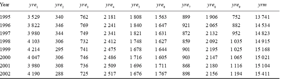
Before the research of income elasticity of the food expenditures, the time dimension of the used database was primarily analysed. No respect of the trends or/and the periodical oscillations in the used CZO database would give the deformed values of the estimated coef-ficients of the income elasticity, the problem of facti-tious regression (Hušek 1932). A set of methods and strategies is defined for the elimination of the factitious regression (Seger, Hindls, Hronová 1998). Within the demand analysis, the seasonality was eliminated by the year aggregation of original quarterly data (yre₁), (yre₂), … , (yre₉), (yrm). The trend components were built in the equation body of the developed de-mand model – the explicit dynamisation of the models in the form (9). The acquired year real levels of the food expenditures (yre₁), (yre₂), … , (yre₉) and the year real amount of money set aside for the food purchases (yrm) are displayed in Table 1.

METHODS OF RESEARCH

The estimations of the income elasticity of the studied food expenditures were based on the system of the nine independent linear-models with the explicit time variable (8). In this system of one-equation models, the income-expenditure relations were defined by means of the fixed base coefficients of percent growths of the household incomes (Krm_t) and the expenditures (Kre_it):

t c Krm b a

Kre_it = _i+ _i× _t+ _i× ; (i = 1, 2, …, 9) (8)

The time variable (t) in the equation system (8) simu-lated the trend development of the used coefficients of growth. For the realised research, the time variable was declared consequently:

t = 1 1995

t = 2 1996

………

t = 8 2002 (9)

The next independent variable (Krm_t) in the designed system of the demand equations (8) represented the fixed-base coefficient of the percentage changes in the real year level of spent amount for foods within the total in-come of the average Czech household. The first year of this time-series (1995) was chosen as the fixed base of the growth coefficients. Thus the growth coefficients were defined as following percentage shares:

100 1 100

1 1

1 _×

   

− = × − =

rm rm rm

rm rm

Krm_t t t ; (t = 1, 2, …, 8)

(10)

The endogenous variable (Kre_it) of the designed mod-el system (8) reflects percentage changes in the real year expenditures of the average Czech household for the food group i. These percentage changes in the studied consumer expenditures were also defined like the fixed-base coefficients with the identical fixed fixed-base term:

100 1 100

1 1

1 _×

   

− = × − =

re re re

re re

Kre_it it it ; (i = 1, 2, …, 9) and (t = 1, 2, …, 8) (11)

The regression parameters (a_i), (b_i), (c_i) in the de-signed dynamical system of the demand linear-models were determined on the base of the ordinary least-squares method. The basic statistical verification of the developed demand models (8) was led through the ob-tained coefficients of determination ( ) and F-tests of its statistical significance ( ). With respect to the aim of the article, T-test of b_i regression parameter ( ) was included too. The details about the used procedures

Table 1. Yearly real expenditures household for foods and yearly real amounts of the average Czech for foods (CZK)

Year yre₁ yre₂ yre₃ yre₄ yre₅ yre₆ yre₇ yre₈ yre₉ yrm

1995 3 529 340 762 2 181 1 808 1 563 899 1 906 752 13 741

1996 3 822 346 769 2 241 1 840 1 647 921 2 065 882 14 534

1997 3 980 344 749 2 341 1 821 1 631 872 2 132 952 14 823

1998 4 103 306 732 2 412 1 748 1 627 859 2 092 1 035 14 915

1999 4 214 295 741 2 475 1 678 1 644 901 2 195 1 025 15 168

2000 4 047 306 746 2 486 1 716 1 605 903 2 147 1 065 15 021

2001 3 980 308 736 2 509 1 696 1 711 868 2 180 1 116 15 104

2002 4 190 288 725 2 517 1 676 1 767 898 2 156 1 194 15 411

2 i R ] [R_i2 F

of the statistical verification are available in Basic Econo-metrics by Gujarati (1988) e.g.

After the parameters quantification of dynamical de-mand system (8) and its statistical verification, the in-come elasticity of the studied groups of food expenditures was evaluated. For the evaluation of the investigated elasticity of expenditures of the average Czech household for the ith _{food groups, the achieved} value of the b_i regression parameter (coefficient) was used:

i i=b

η ; (i = 1, 2, 3, …, 9) (12)

If obtained values of income-expenditure elasticities (12) are supplemented with the significant levels of rele-vant T-tests of b_i regression parameter, then we receive the probability (P) of these point estimations:

[

]

P ; (i = 1, 2, 3, …, 9) (13)

With respect to the consequent adjustments of the in-come-elasticity coefficients (12) to Engel aggregation condition (4), it is useful to determine limits of the esti-mation. For the maximal extent of the coefficient adjust-ing, it is possible to use 95% confidence intervals of the relevant regression parameters(b_i)

05 . 0 1 )] ( )

(

[bi−T_(0,05)/2×sbi ≤ηi≤bi+T_(0,05)/2×sbi = −

P

(i = 1, 2, 3, …, 9) (14)

Thus, the adjusted values of the elasticity coefficient have to lie on the probability level of 95% between the lower (h_i)_L and the higher (h_i)_H limit of the defined confi-dence intervals (Gujarati 1988):

95 . 0 ] ) ( )

[(ηi L≤ηi≤ ηi H =

P ; (i = 1, 2, 3, …, 9) (15)

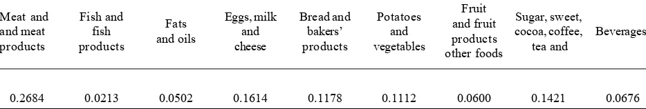
After the outlines of basic statistical aspects of the point estimations of studied elasticity, the obtained values of the income-elasticity coefficients were test-ed by Engel aggregation condition (4). For the realisa-tion of the aggregarealisa-tion test (4), the relevant weights (w_i) were firstly determined by principle (5). The de-signed system of demand model (8) provides the con-stant values of income-expenditure elasticities from 1995 to 2002, so the quantifications of the partial weights were based on its average level within the studied period of eight years (w_i):

∑

∑

= =

= ₈

1 8

1

t t

t it

i

yrm yre

w ; (i = 1, 2, 3, …, 9) (16)

The received weights for the investigated food groups are depicted in Table 2.

The achieved average levels of weights (Table 2.) to-gether with the estimations of income-elasticity coeffi-cients (12) were inserted to the Engel aggregation condition (4), so the theoretical error of estimations (ψ) can be defined:

∑

= η × − =

ψ 9

1

1

i i i

w (17)

The issue of the ψ elimination in the estimated values of income-elasticity coefficients (12) stays the strategy for the separation of adjusted individual coefficients from non-adjusted individual coefficients. In this view, the y distribution among the complete set of the estimated coefficients of income elasticity is mathematically easier cause. The distribution theoretical error of estimation (ψ) can be based on the defined system of the weights (16), thus:

ψ × + + ψ × + ψ × = × ψ =

ψ

∑

= 1 2 9

9

1

... w w

w w i

i (18)

The use of the weight system of Engel aggregation condition (16) for the ψ distribution resulted in the sim-ple patterns for coefficient adjusting:

ψ + η =

ηi)C i

( ; (i = 1, 2, 3, …, 9) (19)

But the realisation of y distribution process (19) is af-fected the one practical disadvantage, that the correct values of the income elasticities are also changed togeth-er with the incorrect estimations of the given coefficients. Because, the value adjusting within a selected subset of obtained coefficients of income elasticity is more suitable for the real analysis of the income-demand elasticity. The subset of the adjusted coefficients can be determined in association with achieved significant level of T-test. The limit value for the definition of studied subset is possible to take the 95% level of T-test significance. Thus, the

Table 2. Average budget shares of yearly real expenditures for foods in order to the total sum of money set aside for total food purchases of average Czech household.

Meat and Fish and Eggs, milk Bread and Potatoes Fruit Sugar, sweet,

and meat fish Fats and bakers’ and and fruit cocoa, coffee, Beverages

products products and oils cheese products vegetables _{other foods}products tea and

value adjusting will be done only for income-elasticity coefficients with the significant level of T-test lesser than 95%.

With respect to the definition criterion, the complete set including 9 coefficients of income-elasticity was di-vided into two parts. The first part of the set contained r of income-elasticity coefficients, which will be adjusted. The extent of this coefficient subset was (1, … , r). The second part of the set included (9 – r) non-adjusted co-efficients of investigated income elasticity, thus extent of the subset was (r + 1, … , 9). The total theoretical error of the elasticity estimations (ψ) was naturally distribut-ed only within the first subset of coefficient set. The subset-bounded process of y distribution was based on the modified system of weights (20):

ψ × + + ψ × + ψ × = × ψ = ψ

∑

∑

∑

∑

∑

(r < n) (20)

Within the given subset, the adjusted values of the income-elasticity coefficients were determined by the formula (21):

∑

( ; (i = 1, 2, …, r); (r < n) (21)

RESULTS AND DISCUSSION

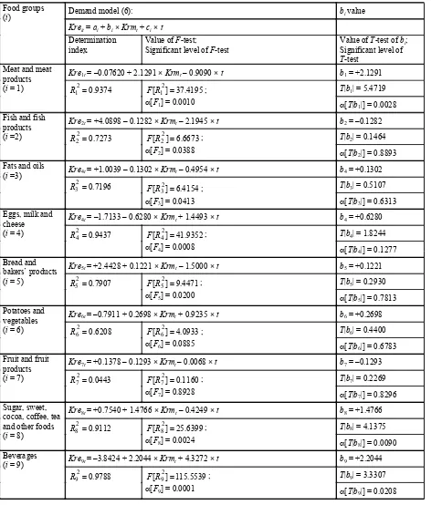
According to the above-described methodology, the income-elasticity research of the food expenditures with-in the average consumer basket of Czech household be-gan by the construction of the demand system of nine independent linear-models with the explicit time variable (8). The individual parameters and the statistical diagnos-tics of the developed models are listed in Table 3.

The results of the significant levels of performed F -tests (in Table 3) clearly demonstrate, that the developed demand system of dynamic linear models (8) is statically significant. Thus, the demand system (9) can be com-pletely used for the quantitative analysis of income elas-ticity in the field of food expenditures of the average Czech household. Maybe only, the individual demand model for fruit and fruit products was not acceptable from that point of statistical diagnostics. The model did not get even the 10% significant level of F-test.

The income elasticity of the expenditure groups within consume basket of the average Czech household was in-vestigated by means of the point estimations of the rele-vant regression parameters (b_i), formula (12). The achieved values of the coefficients together with upper and lower bounds of these estimations are displayed in Table 4.

But the estimated coefficients of income elasticity in Table 4 do not keep the Engel aggregation condition, formula (4):

0.2684 × (+2.1291) + 0.0213 × (–0.1282) +

+ 0.0502 × (–0.1302) +0.1614 × (+0.6280) + 0.1178 × × (+1.1221) + 0.1112 × (+0.2698) + 0.0600 × (–0.1293) + + 0.1421 × (+ 1.4766) + 0.0676 × (+2.2044) = 1.0590 > 1

(22)

For that reason (22), the following research of income elasticity of studied expenditures was focused on adjust-ing of the obtained values of elasticity coefficients (12). In order to adjust the relevant values of elasticity coeffi-cients, the total theoretical error of estimation (y) was firstly determined by the formula (17):

0590 . 0 0590 . 1 1 1 9 1 − = − = η × − = ψ

∑

i i i

w (24)

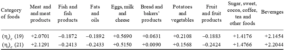
For the distribution of ψ value (24), both described approaches were used. Within the first adjustment meth-od, the distribution process of y was based on the weight system (16). Thus, the distribution of the total theoreti-cal error of estimations ran numeritheoreti-cally by formula (18) for the complete set of income-elasticity coefficients. The adjusted values of all income-elasticity coefficients were determined in accordance with the formula (19). Within the second adjustment method, the distribution process of ψ was based on the modified weight system (20) and was purely applied to the subset of studied elasticity co-efficients with significant level lower than 95%. Within the given subset, the adjusted values of the income-elas-ticity coefficients were calculated by the formula (21). In the investigated group of food expenditures, the coeffi-cient of the income elasticity of the expenditures for fish and fish products, for fat and oils, for eggs, milk and cheeses, for bread and bakers’ products, for potatoes and vegetables, for fruits and fruit products was adjusted. Thus, the value of 6 of 9 elasticity coefficients was ad-justed. On the other hand, 3 coefficients of studied elas-ticity remained aloof the value adjusting. Both levels of results in the field of the coefficient adjusting (19), (21) are depicted in Table 5. In economical interpretations of achieved results, the primary emphasis will lay on the adjusted values of coefficients by the formula (21).

According to the displayed results in Table 5, it is possible to define within the studied component of the consumer basket of the Czech average household the normal (the positive values of income-elasticity coeffi-cients) and the inferior (the negative values of income-elasticity coefficients) groups of foodstuffs. But, this classification of the food groups in the investigated consumer basket has to be taken very reasonably, be-cause the negative values of the income-elasticity co-efficients were found very near to the zero level (less than 0.25%). In the observed period (1995–2002), very weak negative responses to the income changes were especially found in the field of expenditures of the av-erage Czech household for fish and fish products, for fats and oils, and for fruit and fruit products. Within those enumerated groups of the foodstuffs, the rise of

∑

i i i

Table 3. Parameters and statistical diagnostics of the developed demand model

Demand model (6): bi value

Kreit = ai + bi × Krmt + ci × t Food groups

(i)

Determination

index Value of SignificantF-test; level of F-test Value of SignificantT-test of level of bi; T-test

Kre1t = –0.07620 + 2.1291 × Krmt – 0.9090 × t b1 = +2.1291 T|b1| = 5.4719 Meat and meat

products

(i = 1) R₁2=0.9374 4195F[R₁2]=37. ;

α[F1] = 0.0010 α_{[T|b1|] = 0.0028} Kre2t = +4.0898 – 0.1282 × Krmt – 2.1945 × t b2 = –0.1282

T|b2| = 0.1464 Fish and fish

products

(i =2) 2 _0.7273 2 =

R F[R₂2]=6.6673;

α[F2] = 0.0388 α[T|b₂|] = 0.8893 Kre4t = +1.0039 – 0.1302 × Krmt – 0.4954 × t b4 = +0.1302

T|b3| = 0.5107 Fats and oils

(i =3)

7196 . 0

2 3 =

R _[ 2_{] 6.4154}

3 = R

F ;

α[F3] = 0.0413 α[T|b3|] = 0.6313 Kre4t = –1.7133 – 0.6280 × Krmt + 1.4493 × t b4 = +0.6280

T|b4| = 1.8244 Eggs, milk and

cheese

(i = 4) _R42_{=0.9437 F[R4}2_]=41.9352;

α[F4] = 0.0008 α[T|b₄|] = 0.1277 Kre5t = +2.4428 + 0.1221 × Krmt – 1.5000 × t b5 = +0.1221

T|b5| = 0.2930 Bread and

bakers’ products

(i = 5) R₅2=0.7907 F[R₅2]=9.4471;

α[F5] = 0.0200 α_{[T|b5|] = 0.7813} Kre6t = –0.7911 + 0.2698 × Krmt+ 0.9235 × t b6 = +0.2698

T|b6| = 0.4400 Potatoes and

vegetables

(i = 6) 2 _0.6208 6 =

R F[R₆2]=4.0933;

α[F6] = 0.0885 α[T|b₆|] = 0.6783 Kre7t = +0.1378 – 0.1293 × Krmt – 0.0068 × t b7 = –0.1293

T|b7| = 0.2269 Fruit and fruit

products

(i = 7) R₇2=0.0443 F[R₇2]=0.1160;

α[F7] = 0.8928 α_{[T|b7|] = 0.8296} Kre8t = +0.7540 + 1.4766 × Krmt – 0.4249 × t b8 = +1.4766

T|b8| = 4.1375 Sugar, sweet,

cocoa, coffee, tea and other foods

(i = 8) 0.9112

2 8 =

R F[R₈2]=25.6399;

α[F8] = 0.0024 α[T|b₈|] = 0.0090 Kre9t = –3.8424 + 2.2044 × Krmt + 4.3272 × t b9 = +2.2044

T|b9| = 3.3307 Beverages

(i = 9)

9788 . 0

2 9 =

R F[R₉2]=115.5539;

α[F9] = 0.0001 α[T|b₉|] = 0.0208

the real yearly incomes by 1% caused the decrease in the real year level of the food expenditures by approxi-mately 0.24%. In the observed period, other studied groups of food expenditures of the average Czech household achieved entirely positive reaction to the income changes. The positive income responses mani-fested the most intensively in the field of expenditures for beverages and in the field of expenditures for meat and meat products. In both expenditures groups, the

milk and cheeses. In that case, the increase of yearly real level of incomes induced the rise in the given expendi-tures by 0.52%. More and more inelastic normal income-expenditure reactions were determined for potatoes and vegetables, where the rise of the year real income by 1% brought only 0.16% increase in the given expenditure field. And finally, the expenditures of the average Czech household for bread and bakers’ products were found almost without income reactions. The coefficient of in-come elasticity converged to zero level.

CONCLUSION

The realised research was focused on the quantitative analysis of the income elasticity in the field of the food expenditures of the average Czech household between 1995 and 2002. In addition to the quantification of the income elasticity of the analysed expenditures, the arti-cle contains the suggestion of the methodological prin-ciples for the adjustment of income-elasticity coefficients so that Engel aggregation condition was kept. The meth-od of value adjusting can be used for complete set of estimated coefficients of income elasticity or only for their selected subset. According to the adjusted values of the year income-elasticity coefficients, the studied food expenditures included the category of the inferior goods and the normal goods. In the group of the inferi-ors, there were the expenditures for fish and fish prod-ucts, for fats and oils, and for fruit and fruit products. In the group of the normal food goods, there were bread and bakers’ products; potatoes and vegetables; eggs, milk and cheese; sugar, sweet, cocoa, coffee, tea and other foods; meat and meat products; and beverages.

Howev-er, the demonstrated food classification in the investigat-ed consumer basket has to be taken very reasonably, be-cause the negative values of the income-elasticity coefficients were found very near to the zero level (less than 0.25%). Around zero level (0.009%), the positive income elasticity of expenditures for bread and bakers’ products was founded too. The inelastic income reaction was also identified in the field of expenditures for eggs, milk and cheese (0.52%). On the other hand, the strong elastic reactions to the income changes were found for the food groups: sugar, sweet, cocoa, coffee, tea and other foods (1.48%); meat and meat products (2.13%); and beverages (2.20%).

REFERENCES

Browning E.K., Browning J.M. (1992): Microeconomics, Theory and Applications. 4th edition, USA, Harper Collins Publishers, 719 p.; ISBN 0-0673-52142-7.

Denzau A. (1992): Microeconomics Analysis, Markets and Dynamics. USA, IRWIN, 854 p.; ISBN 0-256-07012-1. Gujarati D.N. (1988): Basic Econometrics, 2nd edition. USA,

McGraw-Hill, 705 p.; ISBN 0-07-0255188-6.

Hušek R. (1999): Ekonometrická analýza. 1. vyd. Praha, Eko-press, 303 p.; ISBN 80-86119-19-X.

Koutsoyiannis A. (1979): Modern Microeconomics. 2nd edi-tion. London, The Macmillan Press, 581 p.; ISBN 0-333-25349-3.

Maurice S.CH., Phillips O.R. (1992): Economic Analysis, Theory and Application. 6th edition Boston: Irwin, 738 p.; ISBN 0-256-08209-X.

Nicholson W. (1992): Microeconomic theory, Basic princi-ples and Extensions. 5th edition. USA, Dryden Press, 825 p.; ISBN 0-03055043-2.

Table 5. The adjusted estimations of the income elasticity of food expenditures of the average Czech

Meat and Fish and Fats Eggs, milk Bread and Potatoes Fruit Sugar, sweet, Category

and meat fish and and bakers’ and and fruit cocoa, coffee, Beverages of foods _{products products oils cheese products vegetables products} tea and

other foods

(η_i)_c (19) +2.0701 –0.1872 –0.1892 +0.5690 +0.0631 +0.2108 –0.1883 +1.4176 +2.1454 (ηi)c (21) +2.1291 –0.2413 –0.2433 +0.5150 +0.0090 +0.1568 –0.2424 +1.4766 +2.2044 Table 4. The estimations of the income elasticity of food expenditures of the average Czech upper and lower bounds of these estimations

Meat and Fish and Fats Eggs, milk Bread and Potatoes Fruit Sugar, sweet,

Category _{and meat fish and and bakers’ and and fruit cocoa, coffee, Beverages} of foods _{products products oils cheese products vegetables products} tea and

other foods

Seger J., Hindls R., Hronová S. (1998): Statistika v hospodářství. 1. vyd. Praha, ETC Publishing, edice Manager/Podnikatel, 636 p.; ISBN 80-86006-56-5.

Tiffin A., Tiffin R. (1999): Estimates of food demand elastic-ities for Great Britain, 1972–1994. Journal of Agricultural Economics, 50: 140–147.

Arrived on 31st _{May 2004}

Contact address: