Characterisation and development of a new multi purpose surface analytical instrument

(1)

Characterisation and development of a new multi-purpose

surface analytical instrument.

RIGNALL, Michael.

Available from Sheffield Hallam University Research Archive (SHURA) at:

http://shura.shu.ac.uk/20280/

This document is the author deposited version. You are advised to consult the

publisher's version if you wish to cite from it.

Published version

RIGNALL, Michael. (2000). Characterisation and development of a new

multi-purpose surface analytical instrument. Doctoral, Sheffield Hallam University (United

Kingdom)..

Copyright and re-use policy

(2)

LEARNING CENTRE

CITY CAMPUS, POND STREET,

SHEFFIELD SI 1W3,

1 0 1 6 6 7 4 8 8 0

(3)

ProQuest Number: 10700925

INFORMATION TO ALL USERS

The quality of this reproduction is dependent upon the quality of the copy submitted.

In the unlikely event that the author did not send a com plete manuscript and there are missing pages, these will be noted. Also, if material had to be removed,

a note will indicate the deletion.

uest

ProQuest 10700925

Published by ProQuest LLC(2017). Copyright of the Dissertation is held by the Author.

This work is protected against unauthorized copying under Title 17, United States C ode Microform Edition © ProQuest LLC.

ProQuest LLC.

789 East Eisenhower Parkway P.O. Box 1346

(4)

’Characterisation and development of a

new multi-purpose

surface analytical instrument'

Michael Rignall

A thesis submitted in partial fulfilment of the

requirements of Sheffield Hallam University for the

degree of Doctor of Philosophy.

In collaboration with Kratos Analytical and Oxford

Instruments Micro-Analytical Group.

(5)

(6)

Abstract

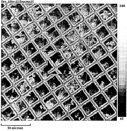
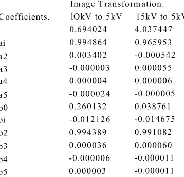
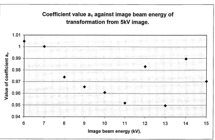
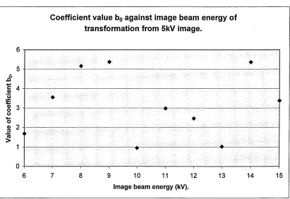
A new multi-purpose surface analytical instrument (the ‘Hallam’ instrument) is described, which combines the surface specific information obtained using x-ray photoelectron spectroscopy (XPS), with bulk information obtained using Energy Dispersive X-ray (EDX) detection. A 15kV electron gun and an ultra high vacuum EDX detector give the instrument an EDX mapping capability. To exploit this to its full potential, spatial alignment of EDX maps acquired at various electron beam energies, E0, was required. The misalignment of images acquired at various E0 values was investigated, and a means of describing the misalignment as a function of E0 was presented. An algorithm was developed which would allow the alignment of offline images acquired at different E0 values. This was demonstrated on images acquired on both the Hallam instrument and on a Phillips XL40 electron microscope.

The small area XPS system developed by Kratos analytical gave a spatial resolution of 30pm at the centre of the field of view, although this deteriorated away from the centre. The reasons for this deterioration in spatial resolution were investigated, and two methods of improving the system were presented. The improvements were implemented on the Hallam instrument and demonstrated using a standard silver grid sample. The small area XPS was applied to a TiAINi coated stainless steel sample to demonstrate its application to real samples, and to display the spatial alignment between the XPS and EDX maps.

(7)

Preface

This thesis, no part of which has been submitted elsewhere, describes the work performed in the Materials Research institute, Sheffield Hallam University, Sheffield, during the period 1995-1998. The work is original and was performed under the supervision of Dr A. Wirth (1995-1997) and Prof. J. Titchmarsh (1997-1998). Where the work of others have aided the investigation, acknowledgements are given. At the request of the industrial partners, no part of this work was published, although a poster titled ‘Calibration and Improvement of an XPS and Small Area XPS system.’ was presented at the 10 the International Conference on Quantitative Surface Analysis (QSA-10).

(8)

Chapter 1 Introduction.

The purpose of this thesis is to explain the development of a multi-technique instrument for the analysis of surfaces, surface coatings and interfaces. The ‘Hallam’ instrument was built as a test bed for a Department of Trade and Industry funded project, as part of the Link Nanotechnology Program. The project, titled ‘Simultaneous Quantitative Thickness Mapping and Chemical Analysis of Thin Films’, was a collaboration between Kratos Analytical, Oxford Instruments Microanalysis Group and Sheffield Hallam University. The project aim was to develop an instrument capable of non-destructive acquisition of quantifiable thickness data, in the range lnm to 5pm.

The ‘Hallam’ instrument is equipped for both surface and bulk analysis techniques. The surface analytical techniques available on the instrument are X-ray Photoelectron Spectroscopy (XPS) and Auger Electron Spectroscopy (AES). Both techniques must be performed within an Ultra High Vacuum (UHV) environment and require high resolution electron spectroscopy. For these reasons it has been common practice among commercial manufacturers to build instruments configured to accommodate both methods. The Kratos Axis-165 is such an instrument and is the foundation of the 'Hallam' instrument that is to be described in this thesis.

X-ray analysis on the scanning electron microscope is a much more widely used analytical tool than surface analysis. While surface analysis was developed to inspect the outermost monolayers of a surface, x-ray analysis is used for the general characterisation and inspection of materials. X-ray analysis is based around the Scanning Electron Microscope (SEM) and thus requires less complicated instrumentation than that used for surface analysis. In order to integrate the components required for x- ray analysis onto the Axis-165, the instrument was reconfigured to accommodate an Energy Dispersive X-ray (EDX )detector and a Backscattered electron detector, which were supplied by Oxford

Instruments. This equipment was specially engineered by Oxford Instruments to be compatible with a UHV environment. A full description of the instrumentation is given in Chapter 3.

The benefits of the project to Oxford Instruments was that thickness mapping by electron probe methods would be developed, and this technique could be directed at the SEM market. The benefits to Kratos were the instrumental improvements which were to be made as part of the project. These included a sample chamber to accommodate an EDX detector, a 25kV field emission electron gun, and a long working distance lens for XPS analysis of thick samples. These features would then be available as options on the Axis-165.

(12)

that during the diagnostic stage, depth profiling XPS (eroding the sample by ion bombardment between XPS analysis) could be used as verification of the non-destructive depth profiling techniques. Oxford Instruments were committing resources to research into thickness mapping, so it was considered that an up to date review of the subject was carried out. This task was undertaken by the author, and a

literature review of thickness mapping by electron probe methods is presented in Chapter 2.

Additional information of film thickness/composition can be obtained by taking EDX measurements at different values of electron beam energy, E0. Oxford Instruments wished to extend their software so this multi kV analysis could be realised. If this data is to be used in the context of mapping then we would wish to obtain spatially resolved information from the same point of a sample at different values of E0. Practically, this requires the registration of SEM images acquired at different values of Eo, and Oxford Instruments requested that this should be investigated by the author. Chapter 4 deals with determining the degree of misalignment between images acquired at different beam energies, and methods of rectifying this misalignment.

An objective of the project was to configure the instrument or create offline procedures to align images acquired from the various techniques. This was necessary to allow verification of non-destructive thickness and compositional mapping, by depth profiling XPS. For these reasons it was decided that scanning small area XPS should align spatially with the other techniques available. The acquisition of spatially resolved XPS data can be achieved using various methods, but that used on the Axis-165 is the sequential pixel by pixel method which shall be described in further detail later. The

instrumentation present on the Axis-165 offers a minimum spatial resolution of 30pm. It is known, however, that this was limited to the centre of the field of view and the image generated by small area XPS was distorted as the distance from the centre of the field of view is increased. It was considered an important part of the project to improve this, and Chapter 5 of this thesis describes this. As this work was carried out by the author, it was considered important that a comprehensive knowledge of spatially resolved XPS was obtained. A review of the literature relevant to this was carried out and is presented in Chapter 2.

(13)

Chapter 2 Theory and Literature Review.

2.0 Introduction

A brief introduction to the two main techniques for which the Hallam instrument is equipped shall be given. The following sections will discuss, in detail, the subjects o f specific interest to this project. These are quantitative x-ray photoelectron spectroscopy , small area x-ray photoelectron spectroscopy and film thickness determination by electron probe x-ray analysis.

2.1 Basic introduction to analytical techniques

2.1.1 X-ray Photoelectron Spectroscopy.

When an x-ray photon interacts with a sample, a photoelectron is ejected. The energy o f the photoelectron depends primarily on the shell from which the electron is ejected. A schematic o f the emission process is shown in Figure 2.1.1 (Watts 1994) for an electron ejected from the k- shell.

Figure 2.1.1.Shematic o f the photo-em ission process. (W atts 1994)

T (Is photoelectron )

vacuum

Fermi level valence band

L>.> L ,

incident x-ray K

The diagram shows the x-ray photon interacting with an electron in the K-shell, causing the emission o f a Is photo-electron. The resulting K shell vacancy is filled by an electron from a higher level which can lead to X-ray fluorescence, or by the radiationless de-excitation process o f Auger emission.

(14)

Ek = h v - E b-<f>

Equation 2.1

[image:14.614.82.459.387.661.2]

There are further terms that may be included in Equation 2.1 but these are small when compared to the uncertainties in the terms shown (Woodruff and Delchar 1994). As the x-ray photon energy (hv) and the work function (j) are known and Ek are determined experimentally, calculation of the electron binding energy is possible. It is the binding energy which defines the element and atomic level from which the photoelectron originated.

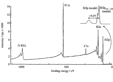
Figure 2.1.2 shows a typical XPS spectrum from Si02 (Drummond 1996). The characteristic XPS core level peaks are super imposed on a background of inelastically scattered electrons. The technique is surface sensitive because only the electrons from the top few nanometers of a surface contribute to these peaks, as those from within the sample would lose kinetic energy by inelastic collisions before leaving the surface of the sample.

Figure 2.1.2 XPS spectrum from Si02. (Drummond 1996)

g

G O

CL

o

14 _{Si2p (oxide) I Si2pI/2 3/2}

I (metal) -4 eV r

12

10

Si2s

8

Si2p

6

O KLL _CIs

4

2

- ■■

0 0

1000 500

hinding energy / eV

(15)

2.1.2. Basic Instrumentation of XPS.

[image:15.613.87.467.369.717.2]

XPS may be considered in simple terms as a primary source of x-rays, a sample, an electron analyser and a detector, all contained within an ultra high vacuum (UHV) enclosure and controlled by a dedicated computer. The need for a UHV environment arises from the surface sensitive nature of the analytical technique. If the sample was not held in UHV conditions then the surface which was being examined would rapidly become contaminated. UHV conditions are usually obtained using ion or diffusion pumps. A simplified schematic of an XPS instrument is shown as Figure 2.1.3.

The x-ray source consists of a filament held at ground potential, and an anode held at high potential (15kV-20kV). The anode material determines the energy of the x-ray radiation, and also the linewidth of the energy. The linewidth of the radiation must not be excessively large so as to widen the resultant XPS peaks. In practice A1 and Mg anodes are used as the x-ray energy (1486.6eV and 1253.6eV, respectively) is high enough to excite most peaks of interest from the elements of the periodic table. If an x-ray source of narrow energy linewidth is required for a high resolution study of XPS peak position and shape, then a monochromator may be employed between the source and the sample.

Figure 2.1.3 Simplified schematic of XPS instrument.

Spectrometer Control Unit.

Channeltron Electron Multiplier.

Hemisp! Sector Analyse

Outer Hemisphere. Inner Hemisphere. ^ Retardation

Lens.

Amplifier. _Analysis Chamber

UHV

Environment.

(16)

Two types of analyser have been used in commercial XPS systems, the concentric hemispherical sector analyser (HSA) and the double pass cylindrical mirror analyser (CMA). The HSA has the higher resolution and is most commonly used in dedicated XPS instruments (Seah 1990b). The electrons pass between inner and outer electrodes which are held at different potentials to disperse the electrons according to energy. To obtain high energy resolution the electrons are retarded to a constant pass energy at which they enter the analyser, the retardation stage consisting of a lens before the analyser entrance slit. The mode of operation is known as fixed analyser transmission mode (FAT). The value of pass energy used may be chosen on the basis of energy resolution and count rate. A channel electron multiplier is usually employed at the exit to the analyser as the electron detector.

2.1.3 Electron probe analysis.

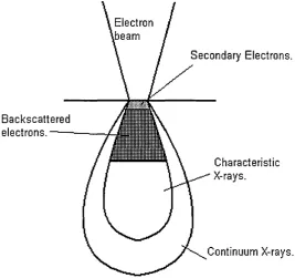
[image:16.614.127.395.386.637.2]

When an electron beam is focused onto a sample surface interactions between the incident electrons and the sample take place, and variety of signals are generated which can be used for analysis. Figure 2.1.4 shows electron beam impinging onto a surface. The signals used in electron probe microanalysis are shown.

Figure 2.1.4. An electron beam impinging on a sample.

Electron .beam

Secondary Electrons.

Backscattered

electrons.---Characteristic X-rays.

Continuum X-rays.

(17)

of the inner energy levels and the vacancy is filled by the transition of an electron from a higher energy level. The wavelength of the characteristic x-ray line is equal to the difference between the energy of the atom in its initial and final states. The x-ray lines are referred to as ‘characteristic’ because the energy of the lines is specific to the emitting element. For each element a number of characteristic x-ray lines exist depending on the possible transitions, and the energy of the incident electron beam. A full explanation of the characteristic x-ray generation is given by Reed (1993a). Electron bombardment also generates continuum or Bremsstrahlung (Reed 1993b). This is generated by electrons decelerating due to collisions with atoms.

If an x-ray spectrometer is used to detect the x-ray emission from a sample then an x-ray spectrum may be recorded consisting of both characteristic and continuum radiation. This spectrum can be used for qualitative analysis as the characteristic peaks identify the elements present in the sample. Quantitative analysis can also be performed as the spectrum may be used to obtain the x-ray intensity for a particular characteristic x-ray line. The concentration of a given element may be determined with an accuracy of 1% if suitable standards are available (Feldman & Mayer 1986).

The x-ray spectrum may be recorded with either a ‘wavelength dispersive’(w.d.) or ‘energy dispersive’(e.d.) spectrometer. The former uses a diffracting crystal which acts as a monochromator, so the x-ray detector sequentially scans through the wavelengths. An e.d. spectrometer records the whole spectrum simultaneously using a solid state x-ray detector. Electronic pulse height analysis is used to sort the pulses produced in the detector according to x- ray energy. Wave dispersive spectrometers produce a much better spectral resolution and peak to background ratio than e.d. spectrometers, but take longer to record a spectrum. As the w.d. spectrometer is an optical system, complicated mechanical arrangements are necessary, which coupled with the need for high quality optics, makes the spectrometer expensive and awkward to fit onto instruments. Energy dispersive spectrometers are commonly used on scanning electron microscopes as little modification to the instrument is necessary. This is the type of spectrometer which was fitted to the Hallam instrument.

(18)

2.2 Quantification of XPS data

2.2.1 Introduction

XPS provides an effective tool for surface analysis o f materials, detecting elements which are present and providing information about the chemical state o f these elements. Quantitative studies are also possible using XPS as a means o f compositional analysis. As surface compositional quantification by XPS is to be used for the project, the theory o f quantification was studied. Further attention was then focussed on the various methods o f characterising the instrument for XPS quantification. As this would have to be done for the Hallam instrument before quantitative studies could be performed, it was necessary to choose which methods should be applied to the Hallam instrument.

2.2.2 Factors affecting quantification

In order to interpret the intensity o f an XPS photoelectron peak we must understand the factors which affect the detection o f the photoelectrons. When irradiated by x-rays, ionisation occurs at the core levels over the depth o f x-ray penetration. The excited electrons are ejected from the surface o f the sample after passing through the solid. The electrons lose energy as they traverse to the surface, so only those from a depth -3A, adjacent to the surface escape to provide the line intensity in the XPS spectrum. Seah (1990c) expressed the intensity o f electrons produced per second from a level X o f an element A as,

n 2k oo oo

A = v A ( h v ) D ( E A ) I \ La(y ) \ U X x y ) s e e S - T ( x y ^ > E A )

oo y =0 0 = 0 y = - oo jc=—oo

x {TV., (

xyz

) exp[- z /

A(E

a) cos

OlflzdydxdOdy

z= 0

Equation 2.2.1

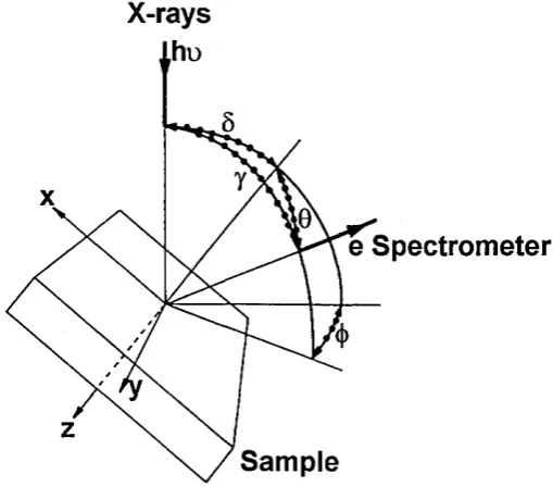
where a ^ (h v ) is the cross-section for emission o f a photoelectron from the relevant inner shell per atom o f A by a photon o f energy hv, D(EyQ is the detection efficiency for each electron transmitted by the electron spectrometer. The geometrical terms which are present in Equation 2.2.1 are shown in Figure 2.2.1. L^(y) is the angular asymmetry o f the intensity o f the

photoemission from each atom, Jo(xy) is the flux o f the X-ray characteristic line per unit area at a point (x,y) on the sample, T(xyyT>E^) is the analyser transmission and N ^(xyz) is the atom density o f the A atoms at xyz. This general equation takes account o f all possible variables which could affect the intensity. Although this equation as written above is not useful for actual

(19)

factors which could determine the detected intensity. The integral over z can be reduced to N^A, (E^)cos0 for a homogeneous solid. I f reference spectra Ira and Irbare taken on the same

instrument, then for a homogeneous binary alloy of elements A and B the intensities can be written as

L U 1 =

h u ;

XAB{EA)XB{EB)

[X

ab

(E

b

)X

a

(Ea)\

R „b ][ N A N m

\ R

raj bN

b4

j

Equation 2.2.2 where Aabis the attenuation length in the alloy, Rrband Rraare roughness's of the pure elemental

[image:19.614.174.429.275.499.2]

standards, and Nrb and Nraare the atom densities in the pure reference materials.

Figure 2.2.1. The geometry of XPS analysis configuration (Seah 1990c).

X-rays

e Spectrometer

Sample

If we ignore the roughness terms and express the matrix term Fabas (Seah 1986)

^ A B ) ^ B C ^ B )

F =

1 AB

and use the expression (Seah 1986)

^ A B ) A a ( E a )

\

aB

I

aA

/

Equation 2.2.3

NM„. X

B RA

B \ a B J

(20)

where aA and aB are the atomic sizes of elements A and B, respectively, the molar concentration of the elements A and B can then be described by the formula

Equation 2.2.5

Assuming the matrix term Fabto be unity would lead to the case where the signal is assumed to be

proportional to molar fractional content. This leads to the general equation

Variations on the above equation are generally quoted as a suitable starting point for quantification. Studies have shown, however, that the value of Fab may scatter around unity

considerably for different alloys (Seah 1980).

Wagner et al (1981) quoted a variation on Equation 2.2.1

where n is the number of atoms per cubic centimetre of the element of interest, f is the flux of X- ray photons impinging on the sample, in units of photon cm 'V1, a is the photo-electric cross section for the particular transition in cm2, (J) is the angular efficiency factor for the instrumental arrangement (angle between photon path and emitted photoelectron), y is the efficiency of production in the photoelectric process to give photoelectrons of normal energy, A is the area of the sample from which photoelectrons can be detected, T is the efficiency of detection of the photo electrons emerging from the sample and X is the mean free path of the photoelectrons in the sample. Although simpler that the equation quoted by Seah, the terms( e.g. y) are less well defined.

Wagner goes on to define the atomic sensitivity factor S as

Equation 2.2.6

I

= nfcxjjyATX

Equation 2.2.7

S

=

crfiyATA

(21)

so for elements A and B of a single binary homogeneous sample

A

B

Equation 2.2.9

This approach contradicts Seah’s claim that matrix effects are of significance although Wagner et al (1980) claims that X A/X B is only slightly matrix dependent. Wagner states that if S is evaluated for each photoelectron line present in the spectra, quantification can be carried out. Wagner’s experimental work concentrated on the evaluation of S for various compounds, each containing either fluorine or potassium. This enabled the sensitivity factor for the other element present in the compound to be expressed relative to the FIs or K2p line. This study was carried out on two instruments producing a set of empirical sensitivity factors still commonly used today. It must be noted that the instruments used both had double cylindrical mirror analysers, as opposed to semi hemispherical analysers. The intensities used in the study were taken from peak area

measurements with straight line background subtraction. This approach is criticised by Seah et al (1984) as much intensity is neglected after background subtraction, which could otherwise be used in quantitative calculations. Figure 2.2.2 shows this.

Figure 2.2.2. The shaded area of the peak is the area contributing to the intensiy after background subtraction.

We shall consider the approach of Wagner as the most convenient, as pure standards are not required for each analysis, but use Seah’s terminology, as it is complete and each term precisely defined. From Equation 2.2.1,if the electron spectrometer has a small entrance aperture and the sample is uniformly illuminated, we get

Intensity

Background

Subtraction

(22)

/, =

<JA(hv

)D(

EA

)LA(r)J(l sec(S)NAM

E Jcosd

XJLL.

T i x y E . M y d x

Equation 2.2.10

We shall consider the case where we need to compare data recorded on the same instrument but from different photoelectron lines. As we shall compare intensities using Equation 2.2.9, many of the terms cancel out. Only those terms with a dependency on photoelectron kinetic energy or atomic number will remain variables. Although the transmission function term, T, is shown as a function of x and y, this is not significant as we assume that the area of analysis remains constant with changes in photoelectron kinetic energy (true for the Axis-165). So for elements A and B of a single binary homogeneous sample

IA nA

a A(

hv

)D(

EA

)LA(r)T(

EA

)Z(

EA

)

IB nBcrB(

hv

)D(

EB

)LB(r)T(

EB

)Z(

EB

)

Equation 2.2.11 The asymmetry terms L is given by (Reilman 1976)

^(r) = l + XA(Ksin27-l)

Equation 2.2.12

The term pA is atomic number dependent, but from Equation 2.2.12, we see that no asymmetry correction is needed for values of y close to 54.7° where L(y)=l. We shall assume this to be the case (true for Axis-165) and incorporate the detection efficiency into the term T(EA) which becomes the transmission function of the whole instrument when operating in wide area XPS mode. In this case Equation 2.2.11 becomes

IA _ nA

<JA(hv

)T(

EA

)M

EA

)

h n B V p S h v ) T ( E B ) M E B )

Equation 2.2.13

So, for the purpose of quantification, we have a sensitivity factor S, expressed as

S

= <

j a

Q

iv

)T{E

a

)X{E

a)

Equation 2.2.14

(23)

A

= c

E~2

+

Equation 2.2.15

where a is the atomic spacing and c and k are constants. Different values o f c and k were given for pure elements, organic and inorganic compounds. A simpler approach is to assume the relation

X = E m

Equation 2.2.16

W agner et al (1980) used experimental data from nine materials to provide a least squares fit, with m in the range 0.54 to 0.81 averaging at 0.66.

The ionisation cross section, a , is defined as the transition probability per unit time for excitation o f a single photoelectron from the core level o f interest under an incident photon flux o f

lc m 'V 1.

Values o f a were calculated by Schofield (1976) for x-ray excitation from magnesium K a lines at 1254eV and aluminium K a lines at 1487eV. The calculations were carried out relativistically using the single potential Hartree-Slater atomic model. The values are published in tabulated form relative to the C Is line. Inaccuracies will arise from using the Hartree-Slater model due to the approximate manner o f treating electron-electron interactions, but an accuracy o f 5% is reported for all except high Z elements.

The term TA is harder to determine as it will vary for individual instruments. It is clear that this must be evaluated experimentally.

2.2.3 Determination of Energy analyser transmission function.

In order to determine the energy analyser transm ission function T(Ek) it is obvious that we must express the intensity o f XPS peaks in terms o f kinetic energy alone. Evaluation o f this is non trivial as the true shape o f XPS spectra (free from instrumental contribution) are difficult to obtain, thus ruling out direct measurement o f intensity as a function o f Ek, the kinetic energy o f the photoelectrons.

(24)

the ratio of the transmission functions for a Perkin Elmer PHI 550 and a VG Scientific ESCA 3 Mk II was proportional to E‘°'244 to an accuracy of 2%. The experiment was extended, and 15 different instruments were calibtated in terms of transmission function, relative to a VG Scientific ESCA 3 Mk II (Seah et al, 1984). The relative transmission fuction for each instrument was expressed as T a En, where n was published for each instrument. Although this this not produce absolute transmission functions, it allowed data from the instruments involved to be compared quantitavely.

The intensity can also be expressed as a function of the analyser pass energy Ep, the energy at which the photoelectrons pass through the analyser after retardation from Ek- Hemminger (1990) proposed the relationship

Peak intensities were taken from a variety of samples with peak positions representing the whole of the 0-1 lOOeV energy range. The spectra were obtained at pass energies 5, 10, 20, 50, 100 and 200eV.

For any given peak the ratio of the peak intensity to the pass energy (I/Ep) was plotted against the pass energy to kinetic energy ratio (Ep/Ek) on log scales. From these plots a relationship of the form

was found for the VG ESCALAB Mkll. This was derived from data taken on three different models of the ESCALAB located in different laboratories, so a large assumption is made by neglecting differences between individual instruments. Strong emphasis is placed on the fact that pass energy and kinetic energy are inseparable. Hemminger claims this enables quantitative comparison of data collected at different pass energies. The primary use of a transmission function is to compare peak intensities acquired with the same conditions. The justification for needing to compare data with different pass energies is that one may be required to use high pass energies when using small area XPS (due to large reduction in intensity) or when measuring minor components of low intensity. Data acquired under these conditions may then require comparison with data acquired under normal conditions at lower pass energy. One would,

I a

E

Equation 2.2.17

(25)

however, avoid this practice as in both cases (small area XPS or minor component measurement) other factors apart from pass energy change would affect quantification.

A simpler method of determining the transmission function of the energy analyser was proposed by Carrazza and Leon (1991). The transmission function was obtained from the dependence of signal intensity on the instrumental pass energy EP, at a given kinetic energy of the incident electrons Ek. The values EP and Ek are related by

Equation 2.2.19

where R is the retarding ratio by which the retarding electrode deccelerates the incident electrons to the pass energy EP before entrance to the dispersive element. In the case of the Hallam

instrument the dispersive element is the semi-hemispherical analyser. For XPS analysis the pass energy remains constant while R is varied (Constant Absolute Resolution). As discussed earlier several experimental variables apart from the kinetic energy of the electrons used (Ek) and the pass energy (EP) influence the transmission function of the instrument. As these experimental variables can be kept constant for XPS measurements, the dependence of the transmission function,T, can be described by

t

=

k ( R y n{

Ek

) ■

Ep

Equation 2.2.20

If we substitute R from Equation 2.2.19 into Equation 2.2.20, the transmission can be represented by

f — y n ? ~ n ( E k ) T ? n ( E k )+ \

1 k p

Equation 2.2.21

Evidently, the value n can be determined at a given Ek by measuring the intensity I at various values of EP. If a plot of the values Log I versus Log EP is generated then the gradient of the straight line fit is equal to n(Ek)+l. This procedure may be repeated for values of Ek across the relevant kinetic energy range, so the value of n as a function of Ek may be established and described by a polynomial such as

n(Ek

)

= a+b

Ek +cEk +dEk

...

(26)

The difference between this method and that proposed by Hemminger is that n is a function of Ek only and not Ep/Ek. The function n(Ek) may be determined for several different modes of

operation such as magnetic or electrostatic magnification and for different entrance aperture settings.

Carrazza used both peak area measurements and background measurements to evaluate the function n(Ek) for a LHS-11 Leybold-Haraeus analyser. From the reported data, the better polynomial fit appears to come from background measurements. XPS Peak intensities are influenced by many parameters (Equation 2.1.1), so will consequently be subject to many uncetainties. Background signal is the result of many interaction within the sample, so

uncertainties will be averaged out. Another advantage of background measurement is that there is no background subtraction method to consider.

The function n(Ek) was applied to quantification using sensitivity factors derived by Equation 2.2.21. Comparison of elemental composition of a catalyst sample was performed, between results when Mg and Al-X-ray sources were used. The results from this showed good agreement which indicated that the validity of Equations 2.2.14 and 2.2.20 is reasonable.

2.2.4 Determination of the instrumental transmission function using the bias method.

This method of determining the instrumental transmission function involves applying a bias voltage to the sample stage relative to ground and was first used by Ebel et al (1983). The mathematical proof of how the transmission function may be derived from measurements taken while the sample is at a bias voltage is presented below (Zommer, 1995).

The measured photoelectron signal intensity at a kinetic energy E may be written as

I{

E

)

= I

„

-T{E

)

-N{E

)

Equation 2.2.23

where Io is the x-ray photon current incident on the sample, T(E) is the instrumental transmission function and N(E) is the energy distribution of electrons from the sample. If a bias voltage Ebias is applied to the sample then the kinetic energy of the electrons entering the analyser will be

E k = E + E b ias. Io is assumed to be a constant value, so can be taken as unity. Equation 2.2.23 can now be written as

I(

Ek,Ebi

as)

= T(

Ek,Ebi

as)

-N(E

)

(27)

which becomes

I (

E + ^bi

as ’ ^

bias

) =

T (

E + ^bi

as

’ E>bi

as

) •

N (

E

)

If we differentiate with respect to Eb we then obtain

Equation 2.2.25

dl

d

E bi

as

d T d

Et

and, since dEii/dEbias==l,

dl

d r

KdE k dE bi

as d

Ebi

asJ

N (

E

)

Equation 2.2.26

Kd

Ek

dEbi

as

j

N ( E

)

d

E bi

as

Equation 2.2.27 Dividing Equation 2.2.27 by Equation 2.2.23 eventually gives the differential equation:

d

In /

d

In

T d\nT

d

E

bi

as

d

E k

dE bi

as

Equation 2.2.28

If we assume that the bias voltage has a negligible effect on the instrumental transmission function, the term d(lnT)/dEb can be neglected. In this case we obtain the differential equation

1

dl

1

dT

1

d

E bi

as

T d

Ek

Equation 2.2.29

the left hand side of Equation 2.2.29 may be established experimentally at different values of kinetic energy E. The relationship between (l/I)dI/dEb and E may be determined and expressed by the polynomial p(E). The solution of Equation 2.2.29 is given by:

T = T0

e x p (jV (£ )c K )

Equation 2.2.30

(28)

T = Ta

exp

(aE

+ bE%

c£% )

Equation 2.2.31

Ebel et al (1983) applied this method to a Kratos XSM 800 instrument and commented on the range o f bias voltages to be used. It is stated that ±100V is suitable but from observation o f analyser transm ission functions (Carrazza and Leon 1991, Hemminger 1990) it is clear that the change in intensity across that range would not be linear. Zommer used -1 0 to+40V bias voltage and claimed successful transmission function determination despite reporting problems with background intensity change.

2.2.5 Development of the metrology spectrometer.

Seah and Smith (1990) approached the problem differently to the methods discussed so far. Their objective was to produce true electron emission spectra for reference samples, which could be used to calculate the transmission function and detector sensitivities o f all instruments. Previous work had shown that the scatter in the ratio o f the XPS intensity o f the Cu 2 p 1/2 and Cu3pi/2 peaks, from different instruments was ±19% (Seah et al 1984). This value was reduced to ±8% when the transmission function o f the analyser was taken into account. This showed that, with simple procedures, reproducible data from the same sample could be obtained in different laboratories. It was envisaged that the reference true electron emission spectra could further increase

reproducibility when applied to all instruments.

To obtain the true electron emission spectra a metrology spectrometer was developed. The instrument was based on a modified VG ESCALAB electron spectrometer. The channel electron multiplier (CEM ) detection assembly was adapted to accommodate a Faraday cup, which was interchangeable with the CEM.

The measured intensity was expressed by

I{E) = I0Q{E)n(

Equation 2.2.32

where n(E) is the absolute spectral intensity (the true electron emission spectra ) from the sample per incident photon as a result o f the basic physical process o f the excitation, transport and emission o f x-ray photoelectrons for the sample, I0 is the x-ray flux and Q(E) represents the effects o f the measurement system. Q(E) is expressed by

Q(E) = H (E)T (E)D(E)F(E)

(29)

where H(E) is the efficiency term representing the effects of the electron detection system, T(E) is the electron optical transmission for the area irradiated, D(E) is the efficiency of the electron detection system and F(E) is the efficiency of the electronics up until the point that the data is recorded.

The instrument could be operated in two modes, constant retard ratio where the energy resolution AE varies with the kinetic energy E but AE/E is constant, or constant pass energy mode where AE is constant. The theory of the transmission function T(E) is covered by Seah and Smith (1990) for each mode of operation, and states that for the constant retard ratio mode the transmission T(E) of photo electrons is proportional to the energy E. In constant pass energy mode the transmission is a more complicated function of energy.

The term H(E) is said to consist of stray magnetic field effects and analyser scattering effects, and it is stated that under certain conditions, such as low retard ratio and small analyser input slit, these effects are negligible. The term F(E) is discussed and is said to be unity as long as the detector discriminators are set correctly and the count rate of the recorded spectra does exceed a value at which pile up would occur. Using these conditions a spectrum is acquired from a sample of copper irradiated by a 5kV electron beam in the constant retard ratio mode. The spectrum is acquired using both the Faraday cup and the CEM detector. As the Faraday cup is assumed to have a detector efficiency D(E)=1 this procedure allows the term for the CEM to be evaluated. Since it is assumed that in constant retard resolution mode T(E) a E, then

for the spectra as long as the precautions listed above are taken.

The instrument is then considered in constant pass energy mode. In this case the terms D(E), H(E) and F(E) are constants as the energy E of the electrons passing through the analyser is constant. The transmission function in this mode is subsequently given by

Equation 2.2.34

(30)

Spectra are then acquired in constant pass energy mode for a variety of pass energies and analyser input slit settings, so T(E) can be evaluated for these conditions. Conventional XPS is then carried out on Cu, Ag and Au reference samples. The evaluated terms of Equation 2.2.33 are applied to the spectra to produce the true electron emission spectra n(E) for that element.

For the true electron emission spectra to be accurate, the transmission function must be accurate. Two factors could influence this. Firstly, if there is any deviation in the theoretical assumption that T(E)aE for the constant retard ratio mode, errors will arise. Secondly, the assumption is that, in constant pass energy mode the term H(E) is constant. This is assumed because of the constant pass energy through the analyser. The factors included in the H(E) term such as stray magnetic field could influence the electrons before they are retarded to the pass energy and enter the analyser.

As a conclusion to this work a so called round robin study was launched to compare the true electron emission spectra of Cu, Ag and Au to spectra acquired on different instruments. The results of this study were subsequently published (Seah 1993). The study involved 25 different instruments from 9 manufacturers. Each participant was instructed to acquire XPS spectra from the Cu, Ag and Au reference samples they were supplied with, under normal operating conditions. Spectra were acquired from 200 to 1600eV kinetic energy with a leV increment. For each instrument used, calibration was accomplished, as the ratio of measured to reference spectra provides the Q(E) function for that instrument.

The study found a large variation in Q(E) for instruments from different laboratories, including variations between the same model operated under identical conditions. This highlights the need for separate and regular calibrations of instruments used for quantitative XPS. The true electron emission spectra were later provided in a standard digital format in a National Physical

Laboratory (NPL) software package, which is described by Seah (1995). The software will compare measured spectra to the reference spectra and also diagnose any problems such as errors in quantification.

2.2.6 Discussion

The study of the factors which effect quantification was useful to the characterisation of the Hallam instrument, as it will enable us to apply quantification to pure samples and compare results for different elements. The study told us which factors were relevant and how these should be derived. In the case where published values should be used, as for the ionisation cross section,

(31)

The spectra derived from measurements on the metrology spectrometer will be used extensively by the surface analysis community. Although the spectra may not truly represent the electron emission spectra, they allow XPS data from different laboratories to be compared. To compare the true emission spectra to spectra taken on the instrument which requires quantification, the digitised spectra must be purchased from the NPL. At the time that the instrument

characterisation work took place this was not available to the author.

A comparison of methods of determining the transmission function was carried out by Weng et al (1993). They used the methods of Hemminger et al (1990), Carrazza and Leon (1991) and a method based on evaluating the terms of Equation 2.2.14. The latter method was unsuccessful as it is difficult to obtain many data points in the Ek range, since each point must be obtained from a measurement of a pure element. It was, however, considered useful for checking the validity of other methods. Weng considered Hemminger's method as the most versatile, as the value of n in Equations 2.2.17 and 2.2.21 is dependent on both Ep and Ek. Weng applied the methods to two instruments, a VG ESCA 3 Mkll and A Scienta X-probe, and concluded that n was constant for the VG instrument and dependent on Ep/EK for the Scienta instrument.

It would seem appropriate for an analyst to determine whether n is constant or dependent on Ek or Ep/EK before choosing which method to use (Hemminger’s or Carrazza’s method). It would be desirable to use the method proposed by Carrazza as this is the simpler and the parameter n can be related to a physical parameter, R, the retard ratio.

(32)

2.3 The Development of Small Area XPS.

2.3.1 Introduction.

XPS was largely assumed to be an area averaging technique. With techniques such as Auger electron spectroscopy and SIMS, where the primary excitation beam consists of charged particles, focussing of the beam to submicron dimensions and rastering of the beam is easily achievable using electron optics.

As this is not possible with the X-rays used for photoelectron spectroscopy, it was not until the early eighties that techniques for area restricted XPS were developed. A number of review papers have been written on this subject, in particular Seah and Smith (1988), Drummond (1992) and Drummond (1996). These papers all cover the topic comprehensively and give a detailed account of the various

methodologies, but can obviously only comment on the technology developed at the time of writing.

There are two approaches to achieving spatially resolved XPS. One is to reduce the size of the X-ray beam, thus using a microprobe to define the area of analysis. The second is to modify the collection electron optics to obtain spatially resolved data. As small area XPS is important to the project we shall examine both cases, so we may be aware of the instrumental options available when constructing a multi-technique instrument. A comprehensive knowledge of the small area XPS may also help us to improve the system on the Hallam instrument.

2.3.2 X-ray Probe Methods

Several methods of generating an X-ray microprobe have been suggested (Seah and Smith 1988). Single or double aperture collomation of the X-ray source is possible but inefficient when applied to XPS. The application of reflecting optics by use of total internal reflection has been applied in x-ray microscopy, but again could not produce the required intensity at the desired spatial resolution.

One method of focussing an X-ray beam is to use the reflecting and diffracting properties of the crystal monochromator (Chaney 1987). The crystal monchromator is primarily used as a means of generating an X-ray beam of characteristic line width <0.4eV, which is free from satellite peaks and

Bremsstrahlung radiation. A crystal monochromator uses a quartz crystal to disperse the X-ray energies by diffraction as predicted by the Bragg equation.

nX

- 2d

- sin#

Equation 2.3.1

(33)

about 0.05% the diameter o f the circle, so it is obvious that the m onochrom ator can provide a route to small area XPS.

Chaney (1987) demonstrated that with careful design a probe size o f 100pm could be attained. Figure 2.3.1 shows the type o f arrangem ent used, which has been com mercially exploited by Fisons in the form o f the S-Probe. An x-y stepper motor is used to scan the sample across the beam to provide imaging capability.

The diameter o f the x-ray beam on the sample is dependent on the size o f the x-ray source spot, which will be the same size o f the electron beam incident on the x-ray source material. The electron beam can be focused to a sub-micron diameter, but must be o f sufficient beam current to provide a useful x-ray flux. Furthermore, the thermal loading produced by the electron beam on the material must not be excessive. Larson and Palmberg (1994) claim anode thermal loadings o f 80kW m m '2 and 1.2kW mm'2 in spot diameters o f 4pm and 250pm respectfully.

The small x-ray spot will be magnified by the crystal and be subject to chromatic, aperture and diffraction aberration. Larson and Palmberg (1994) used a quartz crystal cut parallel to the 1010 plane and bent elliptically to cause non linear spacing o f the lattice planes. This was to com pensate for the aperture aberration, and an x-ray beam diameter o f 10pm on the sample was achieved. Although the monochrom ated small spot produced by the aforementioned methods is o f low intensity, the resultant spectra are o f higher energy resolution and have a higher signal to noise ratio.

Figure 2.3.1 Small x-ray probe generation using a m onchrom ator (W atts 1994b).

hemispherical electron energy analyser

focusing

monochromator crystal

— electron lens photoelectrons

sample

050sample

(150 pm irradiated)

photoelectrons

small area XPS spectrum fast

multichannel

detector

(34)

A number of researchers have used Fresnel zone plates to produce a small diameter x-ray beam,

utilising synchrotron radiation sources to provide the intense x-rays need for this technique. The first of this type of instrument (Ade et al 1990) used a spherical monochromator followed by a focussing zone plate to produce a spot diameter of 0.3pm. The sample is mechanically scanned across the beam allowing the formation of images from photoelectrons detected by a single pass cylindrical mirror analyser, or a more complete spectroscopic examination of a selected area of the sample. It is stated that x-rays between 400 and 800eV may be focussed by the zone plate system, with 670eV radiation used for the example given in the paper, which we presume is the condition for optimum resolution. The problem presented by this is that electrons with binding energy higher than 670eV (plus the work function) will not be ionised, ruling out a significant part of the XPS spectrum. The obvious disadvantage of this type of system is the need for a synchrotron radiation source, which would be prohibitively expensive and impractical for the purpose of XPS alone.

2.3.3. Electro-Optical Methods.

The simplest method of modifying the collection optics to obtain spatially resolved XPS data is to utilise an area restricting aperture (Yates and West 1983). By selecting a small analyser entrance aperture and configuring the transfer lens to magnify the area of analysis on the sample onto the

analyser entrance aperture, small area XPS in the range 102-103pm analysis spot diameter was achieved. The system is shown in Figure 2.3.2.

Figure 2.3.2. Small area XPS using a Limiting Area Aperture (Yates and West 1983).

Retard mesh

.irr-LZ XX V > > ! /*—

( a ) Slit plate ad ju ste r

C hannel electron d e te c to r

( c ) Transfer lens

( b) Lens a p e rtu re

(35)

The procedure was carried out on a multi-technique instrument equipped with a scanning electron gun for Auger analysis. The XPS small spot was spatially aligned using the scanning electron gun as an internal reference. The sample was moved manually to locate the sample area of interest at the small area XPS position.

Figure 2.3.3. Imaging XPS using a pre-lens scanning system. Known as the sequential pixel by pixel method of generating an image (Watts 1994b).

To adapt this system to an imaging system deflection plates were placed between the sample and the lens. By applying voltages to these plates the area selected by the entrance aperture can be scanned across the surface of the sample, and has been implemented on the VG Escalab 2 (Seah and Smith

1988). This type of system may be thought of as an electron microscope in reverse and is commonly known as a virtual microprobe. Figure 2.3.3 shows the pre-lens scanning system. The virtual microprobe can be scanned across the sample surface and the intensity at the detector synchronously monitored to form an image of the distribution of an element or of a particular chemical state. It is also possible to apply point spectroscopy to an area of interest after an image has been acquired.

To further understand how this type of system may be improved upon we must consider the optics. If we examine the system illustrated in Figure 2.3.3, we have a situation where the limiting field aperture is the analyser entrance aperture. If the lens has a magnification M, and the analyser entrance aperture

is of width D, then the width of the area of the sample s which can be seen by the analyser is given by

/i a p e r tu r e

la r g e a r e a X-ray s o u rc e

outpu* slit ano

d e t e c t o r

p r e - l e n s scan n in g sy s tem

s a m p le

D

s

= —

M

(36)

Equation 2.3.2 gives the impression that increasing the magnification and thus reducing the analysis area will reduce the detected intensity, but the transmission of the instrument is further limited by the angular acceptance of the analyser. This shall be expressed by the semi-angle of the beam accepted in the dispersive and non dispersive direction as a s and ps respectively by the expressions

where a 0 and p0 are the limiting half angles and R is the retarding ratio of the lenses.

The intensity of the transmitted photo electrons is given by the proportionality (Seah and Smith 1988)

Hence, the intensity is independent of the magnification, which must be increased if the spatial resolution of the system is to be increased.

Two factors can restrict the implementation of this. Firstly, for XPS it is necessary for the input lens to retard the photoelectrons to the analyser pass energy. If we inspect Equation 2.3.5 it is clear that the need for a sensible retardation ratio will limit the magnification achievable using the input lens. This may be overcome by decoupling the input lens from the probe forming lens.

Secondly, electrostatic lenses suffer from large spherical aberrations (Harting and Reed 1976) which will limit the spatial resolution. These aberrations will increase as the magnification of the probe forming lens is increased.

Equation 2.3.3

and

Equation 2.3.4

Equation 2.3.5

so if we substitute Equations 2.3.3 and 2.3.4 into Equation 2.3.5 we obtain

(37)

In order to increase the magnification of the input lens without introducing large aberrations a radical new design was required. This was provided by Walker (1991) in the form of a single pole piece magnetic lens (Mulvey 1982). Although there was initial hesitancy in introducing a magnetic lens into an XPS instrument, the fact that the lens structure is well clear of the sample («15mm) gave the idea practical credibility, as the lens could reside outside the vacuum. Figure 2.3.4 shows how the lens is incorporated into the instrument. The system shown in Figure 2.3.4 is the system which is used on the Hallam instrument.

Figure 2.3.4. Incorporation of the magnetic lens in the Axis-165 (Drummond 1996).

Energy Analyser.

Detector. Transfer Column.

Area Defining Aperture.

►■^Electrostatic deflection plates.

|._ X-rays.

Image I___

plane. •

Sample.

\

Magnetic Lens.

(38)

2.3.4 Single pole piece magnetic lens.

In general, the smallest aberrations are obtained when lenses are operated in an objective mode w here the specimen is immersed in the imaging field. This is the case with the single pole piece lens, otherwise known as the magnetic imm ersion or “Snorkel” lens. Com pared with other (electrostatic) lens systems in use in other (imaging) XPS instrum ents, its spherical aberration is at least two orders of magnitude smaller. The schematic of Figure 2.3.5 shows the lens operating in standard mode, projecting its imaging field remote from its mechanical structure. This is not the case for conventional magnetic lenses, and so the snorkel lens exhibits a clear advantage for surface analysis because the sample may be supported some distance away from the lens, thus providing a clear line of sight for excitation sources. This is particularly important for high perform ance sources which in general must be placed close to a specimen for optim um specifications.

Figure 2.3.5 Focussing of the magnetic lens.

In detail the snorkel lens consists of an iron circuit with a gap through which extends an iron snout (pole piece). A water cooled solenoid energises the iron circuit to produce an intense m agnetic field between the pole face and the outer body of the lens.

The properties of the snorkel immersion lens may be expressed in term s of the excitation param eter

Angle defining aperture

Pole piece

Magnetic lens iron circuit

...

-— Image plane

(39)

where N is the number of turns in the lens solenoid, I is the current through the solenoid and V is the kinetic energy of the focused electrons. For a given lens pole piece geometry the coil excitation cannot be substantially increased beyond that at which saturation of the lens iron circuit becomes apparent. When iron saturation occurs, the lens iron circuit becomes less efficient at containing the magnetic flux resulting in a loss of the desired optical properties of the lens. However, for optimum optical performance the flux density at the snout must be a maximum, usually limited by the iron saturation value. In practice this is achieved by shaping the pole piece to a specially tapered geometry which ensures that the field in the iron circuit is less than that at the pole face.

All electron optical lenses have aberrations which limit the minimum area which can be clearly defined in the lens object plane (Grivet 1972, Zworykin 1945). The effects of these lens aberrations may be controlled to an acceptable degree by limiting the collection angle of the lens. Reducing the collection angle will also reduce the sensitivity of the detection system introducing signal to noise ratio as another practical limit on minimum area. A selected area diameter may be defined as:

Dl

=dl +dl +dl +dl +dl

Term dg is the Gaussian selected area diameter and is given by:

d = »

g

M

Equation 2.3.8

Equation 2.3.9

Where M is the magnification, and D is the diameter of the selected area aperture diameter. The second term, d s, is the diameter of the disc of least confusion caused by spherical aberration of the lens. This is expressed as:

d s = C J a 3

Equation 2.3.10

where C s is a constant characteristic of lens, and a is the semi collection angle of the lens controlled by an iris in the lens back focal plane, and f is the focal length. The third term dc is the contribution from the chromatic aberration of the lens. This may be expressed as:

d c = C c — f a

E

(40)

where C c is a constant characteristic of the lens, dE is the analyser energy resolution and E is the kinetic energy of the detected photoelectron. Ripple on the lens power supplies can also increase the dc term.

The fourth term da is due to the lens astigmatism and its magnitude depends on the choice of materials, the quality of manufacture of the lens and the alignment of the lens components with respect to the electron optical axis of the instrument (Haine 1961). Contamination of lens components by insulating films and the influence of stray magnetic fields can also cause astigmatism. The final term dd, is the effect of diffraction caused by the finite aperture of the lens and may be expressed as:

dJ

= 0 .6 lf—

Equation 2.3.12

where X is the effective wavelength of the detected photoelectron. Of the above terms, chromatic aberration is less significant than spherical aberration. Lens astigmatism can be reduced to negligible proportions by good design and manufacture, and the effect of diffraction is negligible for the spatial resolutions achievable by XPS. Hence the expression for a selected area diameter becomes

D 2

sa

= d 2 + d 2 + d 2

g s c

Equation 2.3.13

The selected area diameter can be characterised further by

I = 2

.5

f i d

E x d l

a 2

Equation 2.3.14

where I is the detected intensity in counts per second and pdE is the brightness of the emitted photoelectrons from a particular transition with energies between E and E+8E illuminated by a certain x-ray flux. Clearly the value of brightness will depend upon the instrument design and the manner in which it is operated. A typical value for the silver 3d photoelectron peak using MgKa excitation at 450W would be

PdE = 1 0 cps/cm2/rad2/volt

(41)

2.3.5. Alternative methods.

The previously mentioned methods of using electron optics to obtain spatial sensitivity have all used an aperture to limit the area of analysis. Gurker et al (1983) proposed a different method, taking advantage of the dispersive characteristics of the hemispherical analyser. Instead of using an aperture to define the area of analysis they used a narrow slit which is geometrically fixed to lie parallel to the energy dispersive plane of the analyser. A pre analyser magnification of one is used, and post analyser detection is accomplished by microchannel plates followed by a phosphor screen and a TV camera. Figure 2.3.6 shows the analyser arrangement and Figure 2.3.7 shows the image recorded by the TV camera.

Figure 2.3.6 Dispersion within the analyser (Gurker et al 1983).

Specimen Focal plane

(detector)

Figure 2.3.7 Detector image where the information along yD relates to ys (Gurker et al 1983).

2 mm

10

mm-0.5 mm

\ Analysed

specimen area

-25% -50%

-100%

(42)

In one plane of the recorded image we have energy specific information along the direction parallel to the entry slit. The spatial resolution in this direction was 100pm. If one is interested in a given photoelectron species and wants to know its intensity distribution along the analysed line shaped specimen area, the sphere voltage Vs has to be adjusted so that the selected energy band lies within the detector area width xD. Gurker suggested this method could be extended to produce X-Y images with intensity variations of photoelectrons of specific energy. By mechanically scanning the sample along the energy dispersive plane and recording the E-x image at each scan increment the collected information may be decoded to produce an X-Y image at an energy chosen from those in the recorded energy band.

Gurker’s method of obtaining spatial sensitivity has been commercially exploited on the Scienta Esca 300 spectrometer. On this instrument the photoelectron image of the sample is magnified by an Einzel lens (Gelius et al 1990), producing a final resolution of 23pm along the slit direction. The excitation source on this instrument is a highly efficient monochromator, producing an elliptical spot. It is subsequently necessary to include deflection plates above the magnifying lens to align the illuminated sample area with the analyser electron-optical axis. The early models of this instrument did not incorporate imaging, but the equivalent instrument now has this capability, probably due to the falling cost and rising performance of the computation required.

(43)

Figure 2.3.8 Parallel imaging XPS system (Coxon et al 1990).

180° hem i spherical analyser

Hole

S p ectru m de te c to r I Lens 3

Lens 5 Imaging

'ESCA' image

-i x 16 - 3 2

Image x 16 —

Lens 2

Image

d e te c tor 2

Real image 4 x mag

Field a p e r tu re

Lens I

Objective a p e r tu r e

X -rays

HVV*-Spherical Mu-metal chamber

A lens is inserted just before the analyser to convert X-Y information to angular information, and a complementary device at the output stage which re-assembles the energy filtered X-Y image from the angular information. An image resolution of 5pm is attainable using this technique (Coxon et al 1990).

The lenses shown as 3 and 5 use quasi-Fourier transform optics to carry out the conversions. For spectroscopy the area of interest must be mechanically aligned with the electron optical axis and a limiting area aperture introduced. Spectroscopy is then carried out conventionally, as described earlier.

2.3.6 Discussion of various techniques.

(44)

the method used on the Hallam instrument it is clear that the XPS spatial resolution cannot be improved beyond 30 pm.

The E-x method using the entrance slit is less wasteful. The problems here are due to difficulties in generating spectra and images from the E-x maps, although with the increasing speed and capacity of digital hardware, the problem is becoming less significant. Indeed, the combination of this technique with the magnetic lens for initial magnification would, in the authors view, produce the optimum small area XPS system.

(45)

2.4 Thickness Determination By Electron Probe X-ray Analysis.

2.4.1 Introduction

In the following section we shall study the development of thickness determination techniques by x-ray analysis in the electron microscope. The techniques are applicable to both wave dispersive and energy dispersive analysis (WDA and EDA), but greater accuracy is expected with WDA. The use of electron probe microanalysis to determine the thickness of a thin surface layer on a solid substrate has been exploited since the establishment of a linear relationship between layer thickness and the k-ratio parameter. The k-ratio is defined as the x-ray intensity from the film to that from a solid sample of the same element. Early procedures for surface film measurements used empirical calibration of intensity versus thickness (Sweeny et al 1960, Cocket and Davis 1963). To appreciate the development of successive methods we must first understand the generation of characteristic x-rays in a sample irradiated by an electron beam.

2.4.2 The Depth Distribution Function <j>(pz)

X-rays are produced from the surface of the sample down to the maximum depth penetrated by incident electrons before their energy falls below the critical excitation energy Ec of the of the characteristic x- ray line under investigation. Quantitative EPMA analysis requires the calculation of the absorption factor ( as part of the ZAF procedure). For that purpose the production of x-rays as a function of depth must be established. The depth distribution function <j>(pz) represents the x-ray intensity per unit mass depth (pz) relative to that produced in an isolated thin layer. A typical graph of the function cj)(pz) is shown in Figure 2.4.1.

Figure 2.4.1. The <Kpz) curve showing the x-ray intensity from surface layer of thickness Az given by shaded area.

(46)

At the surface of the sample, x-ray emission is enhanced by electrons back-scattered from the bulk of the sample. Hence, the value at the surface, cj)0, known as the surface ionisat