Abstract— In this study, a 3PL multi-product post-sales reverse logistics network is considered which consists of collection centers, repair facilities, production plants, and disposal centers. A bi-objective mixed integer linear programming model is presented for minimizing network design costs as well as minimizing total weighted tardiness of returning products to collection centers. Various decisions including location of repair facilities, repair equipment allocation, and material flows are considered. At the end, a numerical example demonstrates the success of ε-constraint method in obtaining a list of Pareto-optimal solutions for the proposed model.
Index Terms—Mathematical model, Multi-objective optimization, Reverse logistics, Third party logistics service provider
I. INTRODUCTION
URING the past two decades, green supply chain management (GrSCM) has attracted many academics and professionals in logistics and supply chain management. This attraction is highly motivated by three factors including governmental regulations [1], economical benefits of green projects for organizations [2], and finally customers' awareness and nongovernmental organizations [3]. From an operations management perspective, GrSCM models consider the flows from final customers back to the supply chain members such as retailers, collection centers, manufacturers, and disposal centers. One of the most important steps in greening a supply chain is to consider environmental/ecological impacts during logistics network design. This problem, known as the reverse logistics network design problem, is comprised of three main decisions: number and location of facilities specific to a reverse logistics system (e.g. collection centers, recovery facilities, repair facilities, and disposal centers), capacities of facilities, and flows of material. A well-designed reverse logistics network can provide cost savings in reverse logistics operations, help retaining current customers, and attract potential customers [4].
Manuscript received March 23, 2011; revised April 10, 2011.
Seyed Hessameddin Zegordi is with the Department of Industrial Engineering, Faculty of Engineering, Tarbiat Modares University, Tehran, Iran (corresponding author phone: 98-21-88283394; fax: 98-21-88283394; e-mail: [email protected]).
Majid Eskandarpour is with the Department of Industrial Engineering, Faculty of Engineering, Tarbiat Modares University, Tehran, Iran (e-mail: [email protected]).
Ehsan Nikbakhsh is with the Department of Industrial Engineering, Faculty of Engineering, Tarbiat Modares University, Tehran, Iran (e-mail: nikbakhsh@ modares.ac.ir).
In recent years, various researchers have studied the reverse logistics network design problem. For example, Jayaraman et al. [5] proposed heuristics concentration for designing a multi-product 4-tier reverse logistics network design problem. Listeş and Dekker [6] considered a 3-tier reverse logistics network design problem with stochastic demand and supply and developed a scenario-based two-stage stochastic programming model for this problem. In another study, Min et al. [7] developed a mixed integer nonlinear programming model for the two-echelon reverse logistics network design problem for product returns and solved it via a genetic algorithm. Du and Evans [8] considered proposed a hybrid scatter search algorithm for designing a post-sales reverse logistics network consisting of collection centers, repair facilities, and plants for a third party logistics service provider (3PL) with two objectives of minimizing the network total costs and total tardiness of returning products back to collection centers.
In another Study, Demirel and Gokcen [9] considered an integrated remanufacturing reverse logistic network design problem and solved the corresponding model via CPLEX. de Figueiredo and Mayerle [10] proposed a three-stage hybrid heuristic to design a 3-tier reverse logistics network design problem integrated and determine prices of financial incentives for maximizing amount of collected products. Similarly, Aras and Aksen [11] proposed a hybrid tabu search based on Fibonacci search for designing a single echelon reverse logistics network to maximize profits obtained from returned products by customers. Dong [2] modeled a single echelon reverse logistics network for locating hybrid distribution-collection facilities and material flows as a network flow-based deterministic programming model and solved it via a two-stage decomposition heuristic based on location–allocation problem and a revised network flow problem. In addition, Lee and Dong [12] modeled the dynamic design of a reverse logistics network with as a scenario-based two-stage model and solved the proposed model with a hybrid solution method consisting of simulated annealing and sample average approximation. Sasikumar et al. [13] developed a dynamic 7-tier reverse logistics model for maximizing the profits of real-world example of a truck tire-remanufacturing network and solved it via LINGO. Finally, Pishvaee et al. [14] proposed a 4-tier reverse logistics network design model and solved it via a simulated annealing algorithm.
To the best of authors’ knowledge, despite various applications of post-sales networks in real-world situations, the design of post-sales reverse logistics network has received no attention from the researchers except for Du and
A Novel Bi-Objective Multi-Product Post-Sales
Reverse Logistics Network Design Model
Seyed Hessameddin Zegordi, Majid Eskandarpour, and Ehsan Nikbakhsh
Evans [8]. Therefore, in this study, the closed-loop reverse logistics network design problem is considered for a third party logistics service provider providing post-sales services for multiple products belonging to different manufacturers. The network consists of collection centers, repair facilities, production plants, and disposal centers. Multiple decisions including location of repair facilities, allocation of repair equipments, and material flows between different tiers of the reverse logistics system are considered. In addition, various assumptions such as flow of spare parts and new products in the network, limited capacities of plants and repair facilities, and the limit on the maximum number of repair equipments assignable to each repair facility are considered. These assumptions are well matched with characteristics of post-sales service providers for electronics products in which various products designs are similar while the used components are different. For dealing with this problem, a bi-objective mixed integer linear programming model is proposed. In addition, the ε-constraint method is used for obtaining a list of Pareto-optimal solutions for the proposed model.
This paper is organized as follows. In section II, the research problem is defined. The mathematical model for the bi-objective post-sales closed loop reverse logistics network design problem is presented in section III. In section IV, a numerical example is solved for demonstrating the application of the proposed model. Finally, the conclusion and future research directions of this study are given in section V.
II. PROBLEM DEFINITION
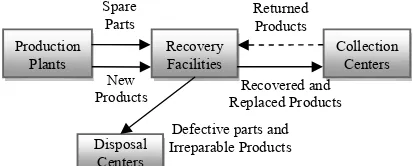
The 4-tier 3PL post-sale reverse logistics network presented in this study consists of production plants, repair facilities, collection centers, and disposal centers (figure 1). A third party logistics service provider (3PL) is responsible for providing the post-sales logistical operations. The 3PL uses its distribution centers and local warehouses as repair facilities and collection centers, respectively.
In this post-sale network, defective products are returned to the collection centers by the customers. Then, the returned products are shipped to repair facilities for initial inspection and repair. The inspection unit in each repair facility is responsible for determining whether a returned product is irreparable or repairable. Irreparable returned products are sent to disposal centers for disposing and the respective customers will be provided with new products as replacements. Repairable returned products are sent to repair facilities for repairing in which the defective parts of repairable products are replaced with necessary spare parts. Then, the repaired returned products are shipped back to the collection centers for delivering to the customers. In addition, the defective parts are shipped to disposal centers for disposal. Finally, the production plants are responsible for providing spare parts and new products for repairing returned products and replacing irreparable returned products, respectively. The material flows in the aforementioned network are demonstrated in figure 1.
In this network, a limited number of equipments with limited repairing capacity are available for repairing the returned products, namely NTmax. In other words, at most,
[image:2.612.312.519.116.199.2]NTmax equipments can be allocated to the repair facilities and each one of equipments can repair a limited number of repairable returned products, namely b. Finally, each candidate repair facility can accommodate a limited number of equipments, namely Nj.
Fig. 1. The research problem post-sale reverse logistics network
III. MATHEMATICAL MODEL
Considering the problem description given in section II, the purpose of the proposed model is the determination of repairing equipment assignment to candidate repair facilities and material flow between collection centers and repair facilities, repair facilities and production plants, and finally repair facilities and disposal centers in order to minimize the fixed costs and transportation costs as well as total tardiness of shipping back returned products to collection center after the necessary operations. For presenting the mathematical model of proposed post-sales reverse logistics network model, the following indices, parameters, and decision variables are considered.
Indices and Parameters:
j: Index of candidate repair facilities, j = 1,…, J,
i : Index of collection centers, i = 1,…, I,
h: Index of plants, h = 1,…, H,
l: Index of disposal centers, l = 1,…, L,
k: Index of products, k = 1,…, K,
b: An equipment repairing capacity expressed in time units,
max
NT : Maximum number of available equipments,
j
N : Maximum number of equipments that can be allocated to jth repair facility,
jk
: Maximum number of kth product type that can be
assigned to jth repair facility,
ik
a : Number of kth product type returned from ith collection
centerto repair facilities, k
t : Amount of time required for repairing a kth product type
at any repair facility, k
: Percentage of irreparable productsfor kth product type,
ij
t : Time required for a round trip between ith collection
center and jth repair facility,
: Maximum allowed time for returning repaired/new products to the collection sites,
hk
: Spare parts capacity of hth plant for kth product type,
ij
cr : Cost of shipping a returned product from ith collection
center to jth repair facility and shipping it back to ith
collection centerafterrepairing/replacing it,
Collection Centers Recovery
Facilities Production
Plants
Disposal Centers
Recovered and Replaced Products Defective parts and Irreparable Products New
Products Spare
hj
cs : Cost of shipping a spare part from hth plant to jth repair
facility for replacing defective parts of repairable products,
hj
cn : Cost of shipping a new product from hth plant to jth
repair facility for replacing irreparable products,
jl
cd : Cost of shipping an irreparable returned product from jth repair facility to disposal center l,
jl
cp : Cost of shipping a defective part of repairable product from jth repair facility to disposal center l,
: Percentage of returned products requiring spare parts,
jn
f : Fixed cost of installing n repairing equipments at jth
repair facility, and
: The exponent measuring the ratio of the incremental to the costs of a unit of equipment representing economies of scale in repair facilities (0 < α < 1).
Decision Variables:
jn
X : Binary variable representing the assignment of n
repairing equipments to jth repair facility,
ijk
Y : Percentage of returned kth product type from the ith
collection center assigned to the jth repair facility,
hjk
W : Amount of spare parts shipped from hth plant to jth
repair facility for repairing repairable kth product type,
hjk
U : Amount of new kth product type shipped from hth
plant to jth repair facility for replacing irreparable products,
jlk
P : Amount of defective parts of repairable kth product
type shipped from jth repair facility to disposal center l, and
jlk
V : Amount of irreparable returned kth product type
shipped from jth repair facility to disposal center l.
Similar to Du and Evan [8], the equipment installing fixed cost scheme originally proposed by Manne [15] is considered. In this scheme, the fixed cost of installing single equipment in the jth facility is assumed to be fj1 b,
where is a constant coefficient, then the fixed cost of installing n equipments in that facility is
1jn j
f nb nb n f . Therefore, the fixed cost
of locating a repair facility at the jth candidate location,
j
FC , can be defined as follows provided that Nj1 jn j X
isat most 1:
1 1 1 2 1
1 1
1
2
j
j
j j j j j j jn
N
j j jN j j
n
j n
FC
FC f X f X ... f n X ... f N X n f X
The Proposed Mathematical Model
Objective function (1) tries to minimize repair equipments fixed installation costs and transportation costs. The transportation costs include costs of shipping 1) products from collection centers to repair facilities and vice versa, 2) spare parts from plants to repair facilities, 3) new products from plants to repair facilities, 4) irreparable returned products from repair facilities to disposal centers, and 5) defective parts of repairable products from repair
facilities to disposal centers.
1 1
1 1 1 1 1
1 1 1 1 1 1
1 1 1 1 1 1
1
1
j
N I J K
J
j jn ij ik ijk
j n i j k
H J K H J K
jh hjk jh hjk
h j k h j k
J L K J L K
jl jlk jl jlk
j l k j l k
Z n f X cr a Z
Z
Y cs W cn U cd V cp P
(1)Objective function (2) minimizes the total weighted tardiness of returning repairable products and new products to the collection centers.
2
1 1 1
Max 0 1
Max 0
I J K
k ij k
ik ijk
i j k ij k
t t ,
Z a Y
t ,
(2)It is noteworthy that due to the nature of equipment allocation scheme, the first objective function tends to allocate the necessary equipments in a centralized manner and the second objective function tends to decentralize the required equipments allocation different repair facilities.
The objective function of the proposed bi-objective mathematical model and its corresponding constraints would be as follows:
1 2
Minimize Z , Z (3)
Subject to: 1 1 j N jn n X
j (4)
1 1 1
1
j N I K
k ik k ijk jn
i k n
a t Y nbX
j (5)1
I
ik ijk jk i
a Y
j , k (6)1 1 j N J jn max j n nX NT
(7)1 1 J ijk j Y
i , k (8)
1 1
1
H I
hjk k ik ijk
h i
W a Y
j , k (9)1 1
H I
hjk k ik ijk
h i
U a Y
j , k (10)1 J hjk hk j W
h , k (11)
1 1
1
L I
jlk k ik ijk
l i
P a Y
j , k (12)1 1
L I
jlk k ik ijk
l i
V a Y
j , k (13)
0 1 jn0
ijk
Y i , j , k (15)
0
jlk
V j , l , k (16)
0
hjk
U h , j , k (17)
Constraint (4) ensures that at most only one of the allowed numbers of equipments is assigned to each repair facility. Constraint (5) limits the time required for repairing products in each repair facility to its corresponding equipments capacity. Constraint (6) limits the maximum number of products assignable to each repair facility for inspection. Constraint (7) limits the sum of number of equipments assigned to repair facilities to the maximum number of equipments available to assign to the repair facilities. Constraint (8) ensures the complete assignment of each collection centers demand to the repair facilities. Constraints (9) and (10) ensure the flow conservation between the plants and the repair facilities for the required spare parts and new products, respectively. Constraint (11) limits the number of spare parts shipping from each plant to the repair facilities considering the plant spare part capacity. Constraints (12) and (13) ensure the flow conservation between the repair facilities and disposal centers for the defective parts of repairable products and irreparable returned products, respectively. Finally, constraints (14-17) define the decision variables types.
Solving the presented model directly via conventional single-objective optimization methods such as branch-and-bound, cutting planes, or benders decomposition is not possible due to the bi-objective nature of the model. Therefore, one has to use a multi-objective optimization technique such as weighted sum, weighted minimax, weighted product, global criterion, ε-constraint, and lexicographic method, [16]. In this study, the ε-constraint [17] is used for transforming the bi-objective optimization problem into a single objective optimization problem.
For illustrating the application of ε-constraint method, consider the following generic bi-objective optimization problem.
1
Minimize f ( X ) (18)
2
Minimize f ( X ) (19)
Subject to:
0 i
g ( X ) i 1,...,m (20) 0
X i 1,...,m (21)
Supposing that f1(X) is the most important objective
function, then one can simply rewrite problem (18-21) as follows to obtain a Pareto-optimal solution [16]:
1
Minimize f ( X ) (22)
Subject to:
2 2
Minimize f ( X ) (23)
0 i
g ( X ) i 1,...,m (24)
0
X i 1,...,m (25) Constraint (23) ensures that the second objective function would not be more than a pre-defined value, ε2. It is
noteworthy that in order to create a list of Pareto-optimal solutions, the above procedure has to be repeated for various values of ε.
IV. NUMERICAL EXAMPLE
In this study, a numerical example was created to evaluate the behavior of the proposed model. For this matter, one random instance of the research problem was generated similar to a generation scheme available in the literature [8]. The nodes of the considered post-sale reverse logistics network were generated on a 100×100 Euclidean space with 20 production plants, 10 repair facilities, 5 collection centers, and 5 disposal centers. In addition, the number of products is considered three. In the randomly generated instance, the number of products returned from each collection center to repair facilities is randomly generated from U[10, 100]. The fixed costs of installing single equipment in each repair facility were generated from the uniform interval of [5b, 10b]. In addition, percentage of
returned products requiring spare parts, the economies of scale in each facility, and maximum allowed time for returning repaired/new products to the collection sites are assumed 0.2, 0.8, and 30, respectively. Other parameters such as facility capacities, transportation costs, and travel times of the considered network are generated according to table I. Finally, necessary mathematical models were coded and solved via commercial optimization software, LINGO 9.0.
TABLEI
PARAMETER GENERATION SCHEME FOR THE NUMERICAL EXAMPLE Parameter Generation Method
tk {8, 10, 12}
γk {0.15, 0.2, 0.25}
σhk U[50,80]
θjk U[400,600]
tij 0.6 × Distance(i,j)
cnhj 0.075 × Distance(h,j)
cdjl 0.05 × Distance(j,l)
crij 0.1× Distance(i,j)
cshj 0.05 × Distance(h,j)
cpjl 0.085 × cdjl
b
1 1 0 3
I K
ik
i k
a
. J
Nj
1 1
1
K J
k k jk
k j
t b
NTmax
1 1 1 1
I K
ik
i k
. a b
Before solving the bi-objective research problem via the ε-constraint method, the ideal points of the network design problem is obtained via single-objective optimization of the research problem (see table II).
TABLEII
IDEAL POINTS OF THE RESEARCH PROBLEM Obj. Function Value Corresponding Obj. Function
Z1 63327.2 8738.88
Z2 1663.27 90708
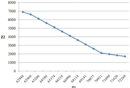
After setting the first objective function to be the most important objective function, the values of ε2 are increased
demonstrate the success of ε-constraint method in creating a list of Pareto-optimal solution as well as the conflict between the two considered objective functions.
Fig. 2. The graph of obtained Pareto-optimal solutions
V. CONCLUSION
One of the most important steps in greening a supply chain is to consider the environmental and ecological impacts of a supply chain during its own initial design stages. In this study, designing a comprehensive model for 3PL multi-product post-sales reverse logistics network consisting of collection centers, repair facilities, production plants, and disposal centers was considered. Various supply chain network design decisions such as location of repair facilities, allocation of repair equipments, and the material flows in the network were considered. These assumptions are well matched with characteristics of post-sales service providers in the electronics industry for products such as cell phones and televisions. For this problem, a bi-objective mixed integer linear programming model was presented. In addition, a numerical example was designed to illustrate the applicability of the ε-constraint method in obtaining a list of Pareto-optimal solutions for the proposed model.
At the end, future research opportunities of this study are integration of the research problem various tactical decisions of the reverse logistics network design, extending the proposed model for incorporating risk and uncertainty via stochastic programming and robust optimization models, and application of metaheuristics specifically evolutionary algorithm with variations of the NSGA algorithm which can be of interest due to their effectiveness in creating a Pareto list.
REFERENCES
[1] J. B. Sheu, "Bargaining framework for competitive green supply chains under governmental financial intervention," Transportation
Research Part E: Logistics and Transportation Review, to be
published, doi:10.1016/j.tre.2010.12.006.
[2] D.-H. Lee and M. Dong, "A heuristic approach to logistics network design for end of lease computer products recovery," Transportation
Research Part E: Logistics and Transportation Review, vol. 44, 2008,
pp. 455-474.
[3] N. Kong, O. Salzmann, U. Steger, and A. Ionescu-Somers, "Moving business/industry towards sustainable consumption: the role of NGOs," European Management Journal, vol. 20, 2002, pp. 109-127. [4] Srivastava, S.K., Network design for reverse logistics," Omega, vol.
36, 2008, pp. 535-548.
[5] Jayaraman, V., R.A. Patterson, and E. Rolland, "The design of reverse distribution networks: Models and solution procedures," European
Journal of Operational Research, vol. 150, 2003, pp. 128-149.
[6] Listeş, O. and R. Dekker, "A stochastic approach to a case study for product recovery network design," European Journal of Operational
Research, vol. 160, 2005, pp. 268-287.
[7] Min, H., H.J. Ko, and C.S. Ko, "A genetic algorithm approach to developing the multi-echelon reverse logistics network for product returns," Omega, vol. 34, 2006, pp. 56-69.
[8] Du, F. and G.W. Evans, "A bi-objective reverse logistics network analysis for post-sale service," Computers & Operations Research, vol. 35, 2008, pp. 2617-2634.
[9] Demirel, N.O. and H. Gökçen, "A mixed integer programming model for remanufacturing in reverse logistics environment," Inrternational
Journal of Advanced Manufacturing Technology, vol. 39, 2008, pp.
1197-1206.
[10] de Figueiredo, J.N. and S.F. Mayerle, "Designing minimum-cost recycling collection networks with required throughput,"
Transportation Research Part E: Logistics and Transportation
Review, vol. 44, 2008, pp. 731-752.
[11] Aras, N. and D. Aksen, "Locating collection centers for distance- and incentive-dependent returns," International Journal of Production
Economics, vol. 111, 2008, pp. 316-333.
[12] Lee, D.-H. and M. Dong, "Dynamic network design for reverse logistics operations under uncertainty," Transportation Research Part
E: Logistics and Transportation Review, vol. 45, 2009, pp. 61-71.
[13] P. Sasikumar, G. Kannan, and A. N. Haq, "A multi-echelon reverse logistics network design for product recovery: a case of truck tire remanufacturing," International Journal of Advanced Manufacturing
Technology, vol. 49, 2010, pp. 1223-1234.
[14] M. S. Pishvaee, K. Kianfar, and B. Karimi, "Reverse logistics network design using simulated annealing," International Journal of Advanced
Manufacturing Technology, vol. 47, , pp. 269-281.
[15] Manne, A., Investments for capacity expansion. Cambridge, MA: MIT
Press, 1967.
[16] Marler, R.T. and J.S. Arora, "Survey of multi-objective optimization methods for engineering," Structural and Multidisciplinary
Optimization, vol. 26, 2004, pp. 369-395.