Using Suffix Arrays to Compute Term
Frequency and Document Frequency for
All Substrings in a Corpus
Mikio Yamamoto*
University of TsukubaKenneth W.
Churcht
AT&T Labs--ResearchBigrams and trigrams are commonly used in statistical natural language processing; this paper will describe techniques for working with much longer n-grams. Suffix arrays (Manber and My- ers 1990) were /irst introduced to compute the frequency and location of a substring (n-gram) in a sequence (corpus) of length N. To compute frequencies over all N(N + 1)/2 substrings in a corpus, the substrings are grouped into a manageable number of equivalence classes. In this way, a prohibitive computation over substrings is reduced to a manageable computation over classes. This paper presents both the algorithms and the code that were used to compute term frequency (tf) and document frequency (dr)for all n-grams in two large corpora, an English corpus of 50 million words of Wall Street Journal and a Japanese corpus of 216 million characters of Mainichi Shimbun.
The second half of the paper uses these frequencies to find "interesting" substrings. Lexi- cographers have been interested in n-grams with high mutual information (MI) where the joint term frequency is higher than what would be expected by chance, assuming that the parts of the n-gram combine independently. Residual inverse document frequency (RIDF) compares docu- ment frequency to another model of chance where terms with a particular term frequency are distributed randomly throughout the collection. MI tends to pick out phrases with noncompo- sitional semantics (which often violate the independence assumption) whereas RIDF tends to highlight technical terminology, names, and good keywords for information retrieval (which tend to exhibit nonrandom distributions over documents). The combination of both MI and RIDF is better than either by itself in a Japanese word extraction task.
1. Introduction
We will use suffix arrays (Manber and Myers 1990) to compute a number of t y p e / t o k e n statistics of interest, including term frequency and document frequency, for all n-grams in large corpora. Type/token statistics model the corpus as a sequence of N tokens (characters, words, terms, n-grams, etc.) drawn from a vocabulary of V types. Different tokenizing rules will be used for different corpora and for different applications. In this work, the English text is tokenized into a sequence of English words delimited by white space and the Japanese text is tokenized into a sequence of Japanese characters (typically one or two bytes each).
Term frequency (tf) is the standard notion of frequency in corpus-based natural language processing (NLP); it counts the number of times that a type ( t e r m / w o r d / n - gram) appears in a corpus. Document frequency (df) is borrowed for the information
Computational Linguistics Volume 27, Number 1
retrieval literature (Sparck Jones 1972); it counts the number of documents that con- tain a type at least once. Term frequency is an integer between 0 and N; document frequency is an integer between 0 and D, the number of documents in the corpus. The statistics, tf and df, and functions of these statistics such as mutual information (MI) and inverse document frequency (IDF), are usually computed over short n-grams such as unigrams, bigrams, and trigrams (substrings of 1-3 tokens) (Charniak 1993; Jelinek 1997). This paper will show how to work with much longer n-grams, including million-grams and even billion-grams.
In corpus-based NLP, term frequencies are often converted into probabilities, using the maximum likelihood estimator (MLE), the Good-Turing method (Katz 1987), or Deleted Interpolation (Jelinek 1997, Chapter 15). These probabilities are used in noisy channel applications such as speech recognition to distinguish more likely sequences from less likely sequences, reducing the search space (perplexity) for the acoustic recognizer. In information retrieval, document frequencies are converted into inverse document frequency (IDF), which plays an important role in term weighting (Sparck Jones 1972).
dr(t) I D F ( t ) = - l o g 2 D
I D F ( t ) can be interpreted as the number of bits of information the system is given if it is told that the document in question contains the term t. Rare terms contribute more bits than common terms.
Mutual information (MI) and residual IDF (RIDF) (Church and Gale 1995) both compare tf and df to what w o u l d be expected b y chance, using two different notions of chance. MI compares the term frequency of an n-gram to what w o u l d be expected if the parts combined independently, whereas RIDF combines the document frequency of a term to what w o u l d be expected if a term with a given term frequency were randomly distributed throughout the collection. MI tends to pick out phrases with noncompo- sitional semantics (which often violate the independence assumption) whereas RIDF tends to highlight technical terminology, names, and good keywords for information retrieval (which tend to exhibit nonrandom distributions over documents).
Assuming a random distribution of a term (Poisson model), the probability p~(k) that a document will have exactly k instances of the term is:
e-O Ok
pa(k) = rc(O,k) - k! '
where 0 = np, n is the average length of a document, and p is the occurrence probability of the term. That is,
N t f tf 8 - -
D N D" Residual IDF is defined as the following formula.
Residual IDF = observed IDF - predicted IDF
df log(1
= - l o g + -
df
----
- l o g ~ +log(1 - e-~)
Yamamoto and Church Term Frequency and Document Frequency for All Substrings
for all substrings in two large corpora, an English corpus of 50 million words of the
Wall Street Journal,
and a Japanese corpus of 216 million characters of theMainichi
Shimbun.
Section 3 uses these frequencies to find "interesting" substrings, where what counts as "interesting" depends on the application. MI finds phrases of interest to lexicog- raphy, general vocabulary whose distribution is far from random combination of the parts, whereas RIDF picks out technical terminology, names, and keywords that are useful for information retrieval, whose distribution over documents is far from uni- form or Poisson. These observations may be particularly useful for a Japanese word extraction task. Sequences of characters that are high in both MI and RIDF are more likely to be words than sequences that are high in just one, which are more likely than sequences that are high in neither.
2. Computing tf and
df
for All Substrings
2.1 Suffix Arrays
This section will introduce an algorithm based on suffix arrays for computing tf and
df
and m a n y functions of these quantities for all substrings in a corpus inO(NlogN)
time, even though there areN(N +
1)/2 such substrings in a corpus of size N. The algorithm groups theN(N +
1)/2 substrings into at most 2N - 1 equivalence classes. By grouping substrings in this way, m a n y of the statistics of interest can be computed over the relatively small number of classes, which is manageable, rather than over the quadratic number of substrings, which would be prohibitive.The suffix array data structure (Manber and Myers 1990) was introduced as a database indexing technique. Suffix arrays can be viewed as a compact representa- tion of suffix trees (McCreight 1976; Ukkonen 1995), a data structure that has been extensively studied over the last thirty years. See Gusfield (1997) for a comprehensive introduction to suffix trees. Hui (1992) shows how to compute
df
for all substrings using generalized suffix trees. The major advantage of suffix arrays over suffix trees is space. The space requirements for suffix trees (but not for suffix arrays) grow with alphabet size: O(N]~]) space, where ]~] is the alphabet size. The dependency on al- phabet size is a serious issue for Japanese. Manber and Myers (1990) reported that suffix arrays are an order of magnitude more efficient in space than suffix trees, even in the case of relatively small alphabet size (IGI = 96). The advantages of suffix arrays over suffix trees become much more significant for larger alphabets such as Japanese characters (and English words).The suffix array data structure makes it convenient to compute the frequency and location of a substring (n-gram) in a long sequence (corpus). The early work was motivated by biological applications such as matching of DNA sequences. Suffix arrays are closely related to PAT arrays (Gonnet, Baeza-Yates, and Snider 1992), which were motivated in part by a project at the University of Waterloo to distribute the
Oxford
English Dictionary
with indexes on CD-ROM. PAT arrays have also been motivated by applications in information retrieval. A similar data structure to suffix arrays was proposed by Nagao and Mori (1994) for processing Japanese text.Computational Linguistics Volume 27, Number 1
it can be just the reverse because there is often an inverse relationship b e t w e e n the size of the alphabet a n d the length of meaningful or interesting substrings. For expository convenience, this section will use the letters of the alphabet,
a-z,
to denote tokens.This section starts b y reviewing the construction of suffix arrays a n d h o w t h e y have been used to compute the frequency a n d locations of a substring in a sequence. We will then s h o w h o w these m e t h o d s can be applied to find not only the frequency of a particular substring b u t also the frequency of all substrings. Finally, the m e t h o d s are generalized to c o m p u t e d o c u m e n t frequencies as well as term frequencies.
A suffix array, s, is an array of all N suffixes, sorted alphabetically. A suffix, s[i], also k n o w n as a semi-infinite string, is a string that starts at position i in the corpus a n d continues to the e n d of the corpus. In practical implementations, it is typically denoted b y a four-byte integer, i. In this way, a small (constant) a m o u n t of space is used to represent a v e r y long substring, w h i c h one m i g h t have t h o u g h t w o u l d require N space.
A substring,
sub(i,j),
is a prefix of a suffix. That is,sub(i,j),
is the first j characters of the suffixs[i]. The
corpus containsN ( N +
1)/2 substrings.The algorithm, s u f f i x _ a r r a y , presented below takes a corpus a n d its length N as input, a n d outputs the suffix array, s.
s u f f i x _ a r r a y *--
function(corpus, N){
Initialize s to be a vector of integers from 0 to N - 1. Let each integer denote a suffix starting at
s[i] in
thecorpus.
Sort s so that the suffixes are in alphabetical order. Return s. }
The C p r o g r a m below implements this algorithm.
char *corpus ;
int suffix_compare(int *a, int *b)
{ return strcmp(corpus+*a, corpus+*b);}
int *suffix_array(int n){
int i, *s = (int *)malloc(n*sizeof(int));
for(i=O; i < n; i++) s[i] = i; /* initialize */
qsort(s, n, sizeof(int), suffix_compare); /* sort */
return s;}
Figures i a n d 2 illustrate a simple example where the corpus ("to_be_ormot_to_be") consists of N = 18 (19 bytes): 13 alphabetic characters plus 5 spaces (and 1 null termination). The C p r o g r a m (above) starts b y allocating m e m o r y for the suffix array (18 integers of 4 bytes each). The suffix array is initialized to the integers from 0 to 17. Finally, the suffix array is sorted b y alphabetical order. The suffix array after initialization is s h o w n in Figure 1. The suffix array after sorting is s h o w n in Figure 2.
As m e n t i o n e d above, suffix arrays were designed to m a k e it easy to c o m p u t e the frequency
(tf)
a n d locations of a substring (n-gram or term) in a sequence (corpus). Given a substring or term, t, a binary search is used to find the first a n d last suffix that start w i t h t. Lets[i]
be the first such suffix a n d s~] be the last such suffix. Then tf(t) = j - i + 1 a n d the term is located at positions: {s[i],s[i +
1] . . . . ,s~]}, a n d o n l y these positions.Yamamoto and Church Term Frequency and Document Frequency for All Substrings
I n p u t c o r p u s : " t o _ b e _ o r _ n o t _ t o _ b e "
Position: Characters: Initialized Suffix Array
s[O] 0 s[l]
1
s [ 2 ]
2
s [ 3 ]
3
s [ 1 3 ] 13
s [ 1 8 ] 14
s [15]
15
s [16]
15
s [ 1 7 ] 17
0 1 2 3 4 5 6 7 8 9 10 11 12 13 14 15 16 17
Itlol_lblel_lolrl_lnloltl_ltlol_lblel
.~"
: : : : ""{ i i i !
' ' ' ! Suffixes d e n o t e d by s [ i ] i i i i i
-" /
."
/ t o b~ o~ n o t t o b~ I /
/
i i i
.... .. j...: o
or
to
j :" ' i i ' '
I
...
" ..,'" I be o rn o t t o be I ." /
/ /
/
I " ~
be o r N o t _ t o _ b e ... ,'"'" ...'/" .y ./" /
Figure 1
Illustration of a suffix array, s, that has just been initialized a n d not yet sorted. Each element in the suffix array, s[i], is an integer denoting a suffix or a semi-infinite string, starting at
position i in the corpus and extending to the end of the corpus.
S u f f i x A r r a y
s[0] 1151
s [1]
2.,
s[2] 8 s[3]
5
s [4] 12
s [5] 16
s [ 6 ]
3
s [7] 17
s [8]
4
s [ 9 ]
9
s [ 1 0 ] 14
s i l l ]
1
s [ 1 2 ]
6
s[13]
10
s [ 1 4 ]
7
s [ 1 5 ] 11
s [ 1 6 ] 13
s[17] 0
Figure 2
S u f f i x e s d e n o t e d b y s [ i ]
_ D e
b e _ o r _ n o t _ t o _ b e _ n o t to b e
_ o r _ n o t _ t o _ b e _ t o _ b e
b e
b e _ o r _ n o t_t o _ b e e
e _ o r _ n o t_t o _ b e n o t _ t o _ b e
o b e
o b e o r _ n o t _ t o _ b e o r _ n o t to b e
o t _ t o _ b e r _ n o t _ t o _ b e t to b e t o _ b e
to b e o r _ n o t _ t o _ b e
[image:5.468.40.373.85.279.2] [image:5.468.39.239.336.628.2]Computational Linguistics Volume 27, Number 1
suffix to start with this term. Consequently, tf("to_be") = 1 7 - 1 6 + 1 = 2. Moreover, the term appears at
positions("to_be")
= {s[16], s[17] } = {13, 0}, and only these positions. Similarly, the substring "to" has the same tf andpositions,
as do the substrings, "to_" and "to_b". Although there may beN(N +
1)/2 ways to pick i and j, it will turn out that we need only consider 2N - 1 of them when computing tf for all substrings.Nagao and Mori (1994) ran this procedure quite successfully on a large corpus of Japanese text. They report that it takes
O(NlogN)
time, assuming that the sort step performsO(N
log N) comparisons, and that each comparison takes constant time. While these are often reasonable assumptions, we have found that if the corpus con- tains long repeated substrings (e.g., duplicated articles), as our English corpus does (Paul and Baker 1992), then the sort can consume quadratic time, since each compar- ison can take order N time. Like Nagao and Mori (1994), we were also able to apply this procedure quite successfully to our Japanese corpus, but for the English corpus, after 50 hours of CPU time, we gave up and turned to Manber and Myers's (1990) al- gorithm, which took only two hours. 1 Manber and Myers' algorithm uses some clever, but difficult to describe, techniques to achieveO(N
log N) time, even for a corpus with long repeated substrings. For a corpus that w o u l d otherwise consume quadratic time, the Manber and Myers algorithm is well worth the effort, but otherwise, the procedure described above is simpler, and can even be a bit faster.The "to_be_or_not_to_be" example used the standard English alphabet (one byte per character). As mentioned above, suffix arrays can be generalized in a straightforward w a y to work with larger alphabets such as Japanese (typically two bytes per character). In the experimental section (Section 3), we use an open-ended set of English words as the alphabet. Each token (English word) is represented as a four-byte pointer into a symbol table (dictionary). The corpus "to_be_or_not_to_be", for example, is tokenized into six tokens: "to", "be", "or", "not", "to", and "be", where each token is represented as a four-byte pointer into a dictionary.
2.2 Longest C o m m o n Prefixes (LCPs)
Algorithms from the suffix array literature make use of an auxiliary array for storing LCPs (longest common prefixes). The
lcp
array contains N + 1 integers. Each element,lcp[i],
indicates the length of the common prefix betweens[i -
1] ands[i].
We pad thelcp
vector with zeros(lcp[O] = lcp[N]
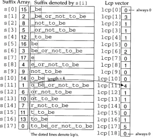
= 0) to simplify the discussion. The padding avoids the need to test for certain end conditions.Figure 3 shows the
lcp
vector for the suffix array of "to_be_or_not_to_be". For example, since s[10] and s[11] both start with the substring "o_be",lcp[11]
is set to 4, the length of the longest common prefix. Manber and Myers (1990) use theIcp
vector in their O ( P + l o g N) algorithm for computing the frequency and location of a substring of length P in a sequence of length N. They showed that theIcp
vector can be computedin O(N
log N) time. These algorithms are much faster than the obvious straightforward implementation when the corpus contains long repeated substrings, though for many corpora, the complications required to avoid quadratic behavior are unnecessary.2.3 Classes of Substrings
Thus far we have seen how to compute
tf
for a single n-gram, but how do we computetf
anddf
for all n-grams? As mentioned above, theN(N +
1)/2 substrings will be clustered into a relatively small number of classes, and then the statistics will beYamamoto and Church Term Frequency and Document Frequency for All Substrings
c o m p u t e d o v e r the classes r a t h e r t h a n o v e r the substrings, w h i c h w o u l d b e prohibitive. The r e d u c t i o n of the c o m p u t a t i o n o v e r s u b s t r i n g s to a c o m p u t a t i o n o v e r classes is m a d e possible b y four properties.
Properties 1-2: all s u b s t r i n g s in a class h a v e the s a m e statistics (at least for the statistics of interest, n a m e l y tf a n d dJ),
Property 3: the set of all substrings is p a r t i t i o n e d b y the classes, a n d
Property 4: there are m a n y f e w e r classes (order N) t h a n substrings (order N2).
Classes are d e f i n e d in t e r m s of intervals. Let
(i,j)
b e a n interval on the suffix array, s[i],s[i +
1] . . .s~]. Class((i,j))
is the set of s u b s t r i n g s that start e v e r y suffix w i t h i n the interval a n d n o suffix o u t s i d e the interval. It follows f r o m this construction that all substrings in a class h a v e tf = j - i + 1.The set of s u b s t r i n g s in a class can b e c o n s t r u c t e d f r o m the
lcp
vector:class((i,j)) = {s[i]ml max(Icp[i], lcp~ +
1])< m ~ min(lcp[i +
1],lcp[i +
2] . . .lcp~'])},
w h e r es[i]m
d e n o t e s the first m characters of the suffixs[i].
We will refer tolcp[i]
a n dIcp~+l]
as b o u n d i n g lcps a n dIcp[i+l], lcp[i+2]
. . .lcp~]
as i n t e r i o r lcps. The e q u a t i o nSuffix A r r a y i Suffix d e n o t e d b y s [ i ]
s[O] 15 _be;
s[l] 2 _ b ~ _ o r _ n o t to be s[2] 8 _}not to be
s[3] 5 --] b r n o t to b e
--s[4] 12 :--to_be
s[5] IB ibei
s[6] 3 :he'or_not to be
s[7]
s [8] i e~_or_not to be s [ 9 ] n o t _ t o _ b e
s [I0] o _ b 4 l e n ~ = 4
sill] ~ or n o t to be s[12] q r _ n o t to be s[13] q't to be s[14] r _ n o t to be s[15] tJ to be s [ 16 ] rio_be,
s [ 17 ] to_be[~or_not to b e
[image:7.468.34.358.327.600.2]The doted lines denote lcp's.
Figure 3
Lcp vector i c p [ O O" icp [i 3 icp [2 I icp [3 I Icp [4 I i c p [ 5 0 icp[6] 2 icp[7] 0 icp[8] I Icp[9] 0 icp[lO] 0
l c p [ 1 2 ] 1
Icp[13] 1
icp [14] 0 icp[15] 0 icp[16] I icp[17] 5 icp[18] O-
-- always 0
always 0
The longest common prefix is a vector of N + 1 integers,
lcp[i]
denotes the length of the common prefix between the suffixs[i -
1] and the suffixs[i].
Thus, for example, s[10] and s[11] share a common prefix of four characters, and thereforelcp[11]
= 4. The common prefix is highlighted by a dotted line in the suffix array. The suffix array is the same as in the previous figure.Computational Linguistics Volume 27, Number 1
Vertical lines d e n o t e lcps. G r a y area d e n o t e s B o u n d a r i e s e n d p o i n t s of s u b s t r i n g s in class(<10,11>).
S [9]lli'
n o t
to be
~'~f7 ° f < 1 0 ' l l > I,Ill 0 __ b e - ~ X<";flO,11> . . . /s [
10 ]
s[ll]]~o]_ b el_or_not_to_be ~1 4_ I
s[12]I lo:;Ir n ~ t to be
...
<10,13>
s[14]s[13]]i!I~to ~-t~_be
e
...
~
B o u n d i n g lcps, LBL, SIL, Interior lcp of <10,11>
L C P - d e l i m i t e d Class interval
<10,11> <10,13> <9,9> <10,10> <11,11> <12,12> <13,13> <14,14>
LBL SIL
Figure 4
{"O_", "o_b", "o_be"} 1 4 {"o"} 0 1 {"n", "no", "not", ...} 0 infinity
{} 4 infinity
{ " o _ b e _ " , " o _ b e o " , . . . } 4 infinity {"or", "or_", "or_n", ...} 1 infinity {"ot", "ot_", "oCt", ...} 1 infinity "r", "r " " _ , r _ n , . . . } " 0 infinity
tf
Six suffixes are copied from Figure 3, s[9]-s[14], along with eight of their lcp-delimited intervals. Two of the lcp-delimited intervals are nontrivial (tf > 1), and six are trivial (tf = 1). Intervals are associated with classes, sets of substrings. These substrings start every suffix within the interval and no suffix outside the interval. All of the substrings within a class have the same term frequency (and document frequency).
above can be rewritten as
class((i, jl ) = {s[i]mlLBL((i, jl) < m <_ SIL((i, jl)}, where LBL (longest bounding lcp) is
L B L ( ( i , j ) ) = max(lcp[i], lcp~ + 1]), and SIL (shortest interior lcp) is
sIn((i,j)) = min(lcp[i + 1], Icp[i + 2] . . . lcp~]).
By construction, the class will be empty unless there is some room for m between the LBL and SIL. We say that an interval is lcp-delimited when this room exists (that is, L B L < SIL). Except for trivial intervals where tf = 1 (see below), classes are nonempty iff the interval is lcp-delimited. Moreover, the number of substrings in a nontrivial class depends on the amount of room between the LBL and the SIL. That is, [class((i,j))l = SIL((i,j)) - LBL((i,j)).
[image:8.468.53.361.56.358.2]Yamamoto and Church Term Frequency and Document Frequency for All Substrings
b o u n d i n g lcps, a n d thin vertical lines denote interior lcps (there is only one interior lcp in this case). The interval {10, 11 / is lcp-delimited because the b o u n d i n g lcps,
Icp[lO] --= 0
a n dlcp[12]
= 1, are smaller t h a n the interior lcp,lcp[11]
= 4. That is, the LBL (= 1) is less than the SIL (= 4). Thus there is room for m between the LBL of s[10]m a n d the SIL of s[10]m. The endpoints m between LBL a n d SIL are highlighted in gray. The class is nonempty. Its size d e p e n d s on the w i d t h of the gray area:class((lO,
11)) = {s[10]mll < m _< 4} = {"o_", "o_b", "o_be"}. These substrings have the same tf: tf = j - i + 1 = 11 - 10 + 1 = 2. Each of these substrings occurs exactly twice in the corpus.Every substring in the class starts every suffix in the interval (10,11), a n d no suffix outside (10,11). In particular, the substring "o" is excluded from the class, because it is shared b y suffixes outside the interval, n a m e l y s[12] a n d s[13]. The longer substring, "o_be_", is excluded from the class because it is not shared b y s[10], a suffix within the interval.
We call an interval trivial if the interval starts a n d ends at the same place: (i, i). The remaining six intervals m e n t i o n e d in Figure 4 are trivial intervals. We call the class of a trivial interval a trivial class. As in the nontrivial case, the class contains all (and only) the substrings that start every suffix within the interval a n d no suf- fix outside the interval. We can express the class of a trivial interval,
class((i, i)),
as{s[i]m]LBL < m <_ SIL}. The
trivial case is the same as the nontrivial case, except that the SIL of a trivial interval is defined to be infinite. As a result, trivial classes are usually quite large, because t h e y contain all prefixes of s[i] that are longer than the LBL. They cover all (and only) the substrings with tf = 1, typically the bulk of theN ( N +
1)/2 substrings in a corpus. The trivial class of the interval (11,11), for example, contains 13 substrings: "o_be_", "o_be_o", "o_be_or", a n d so on. Of course, there are some exceptions: the trivial class,class((lO,
10)), in Figure 4, for example, is very small (= e m p t y set).Not every interval is lcp-delimited. The interval, I l l , 12), for example, is n o t lcp- delimited because there is no room for m of s[ll]m between the LBL (= 4) a n d the SIL (= 1). W h e n the interval is n o t lcp-delimited, the class is empty. There are no substrings starting all the suffixes within the interval (11,12), a n d not starting a n y suffix outside the interval.
It is possible for lcp-delimited intervals to be nested, as in the case of (10,11) and (10, 13). We say that one interval
(i,j)
is nested within another(u,v)
if i < u < v < j (and(i,j) ~ (u, v)).
Nested intervals have distinct SILs a n d disjoint classes. (Two classes are disjoint if the corresponding sets of substrings are disjoint.) 2 The substrings in the class of the nested interval, (u, v), are longer than the substrings in the class of the outer interval,(i,j).
A l t h o u g h it is possible for lcp-delimited intervals to be nested, it is not possible for lcp-delimited intervals to overlap. We say that one nontrivial interval Ca, b) overlaps another nontrivial interval (c, d) if a < c < b < d. If two intervals overlap, then at least one of the intervals is not lcp-delimited a n d has an e m p t y class. If an interval (a, b) is lcp-delimited, an overlapped interval
(c, d)
is not lcp-delimited. Because a b o u n d i n g lcp of /a, b) m u s t be within (c, d) a n d an interior lcp of (a, b) m u s t be a b o u n d i n g lcp of(c,d), SIL((c,d)) <_ LBL((a,b)) <_ SIL((a,b)) <_ LBL((c,d)).
That is, the overlapped interval (c, d) is not lcp-delimited. The fact that lcp-delimited intervals are nested a n d do not overlap will turn out to be convenient for e n u m e r a t i n g lcp-delimited intervals.Computational Linguistics Volume 27, Number 1
2.4 Four Properties
As m e n t i o n e d above, classes are constructed so that it is practical to r e d u c e the com- p u t a t i o n of various statistics over substrings to a c o m p u t a t i o n over classes. This sub- section will discuss four p r o p e r t i e s of classes that help m a k e this r e d u c t i o n feasible.
The first t w o p r o p e r t i e s are c o n v e n i e n t because they allow us to associate
tf
a n ddf
w i t h classes rather than w i t h substrings. The substrings in a class all h a v e the sametf
v a l u e ( p r o p e r t y 1) a n d the samedf
v a l u e ( p r o p e r t y 2). That is, if Sl a n d s2 are t w o substrings inclass((i,j))
t h e nProperty 1:
tf(sl)
= t f ( s 2 ) =j - i + 1
P r o p e r t y 2:
dr(s1)
=rid(s2 ).
Both of these p r o p e r t i e s follow s t r a i g h t f o r w a r d l y from the construction of intervals. The v a l u e of
tf
is a simple function of the endpoints; the calculation ofdf
is m o r e complicated a n d will be discussed in Section 2.6. Whiletf
a n ddf
treat each m e m b e r of a class as equivalent, not all statistics do. M u t u a l i n f o r m a t i o n (MI) is an i m p o r t a n t c o u n t e r example; in m o s t cases,MI(sl) ~ MI(s2).
The third p r o p e r t y is c o n v e n i e n t because it allows us to iterate o v e r classes r a t h e r than substrings, w i t h o u t w o r r y i n g a b o u t missing a n y of the substrings.
P r o p e r t y 3: The classes partition the set of all substrings.
There are t w o parts to this argument: e v e r y substring belongs to at m o s t one class ( p r o p e r t y 3a), a n d e v e r y substring belongs to at least one class ( p r o p e r t y 3b).
Demonstration of property 3a (proof b y contradiction): S u p p o s e there is a sub- string, s, that is a m e m b e r of t w o distinct classes:
class((i,j})
a n dclass((u,v)).
There are three possibilities: one interval p r e c e d e s the other, t h e y are p r o p e r l y nested, or they overlap. In all three cases, s c a n n o t be a m e m b e r of b o t h classes. If one interval precedes the other, t h e n there m u s t be a b o u n d i n g lcp b e t w e e n the t w o intervals w h i c h is shorter t h a n s. A n d therefore, s cannot be in b o t h classes. The nesting case was m e n - tioned p r e v i o u s l y w h e r e it was n o t e d that n e s t e d intervals h a v e disjoint classes. The o v e r l a p p i n g case was also discussed p r e v i o u s l y w h e r e it was n o t e d that t w o overlap- ping intervals c a n n o t b o t h be lcp-delimited, a n d therefore at least one of the classes w o u l d h a v e to be empty.Demonstration of property 3b (constructive argument): Let s be an arbitrary sub- string in the corpus. There will be at least one suffix in the suffix a r r a y that starts w i t h s. Let i be the first such suffix a n d let j be the last such suffix. By construction, the interval
(i,j}
is lcp-delimited(LBL((i,j}) <
Is I a n dSIL((i,j}) >__
Is[), a n d therefore, s is an e l e m e n t ofclass((i,j}).
Finally, as m e n t i o n e d above, c o m p u t i n g o v e r classes is m u c h m o r e efficient t h a n c o m p u t i n g o v e r the substrings themselves because there are m a n y f e w e r classes (at m o s t 2N - 1) t h a n substrings
(N(N +
1)/2).Property 4: There are at m o s t N n o n e m p t y classes w i t h tf = 1 a n d at m o s t N - 1 n o n e m p t y classes w i t h tf > 1.
The first clause is relatively straightforward. There are N trivial intervals (i, i/. These are all a n d o n l y the intervals w i t h
tf
= 1. By construction, these intervals are lcp-delimited, t h o u g h it is possible that a few of the classes c o u l d be empty.To a r g u e the s e c o n d clause, w e m a k e use of a u n i q u e n e s s p r o p e r t y : an lcp- delimited interval
(i, jl
can be u n i q u e l y d e t e r m i n e d b y an SIL a n d a representative ele-Yamamoto and Church Term Frequency and Document Frequency for All Substrings
m e n t k, where i < k < j. For convenience, we will choose k such that
SIL(<i,j>) = Icp[k],
but we could have uniquely determined the lcp-delimited interval b y choosing a n y k such that i < k G j.
The uniqueness property can be d e m o n s t r a t e d using a proof b y contradiction. Suppose there were two distinct lcp-delimited intervals,
<i,j>
a n d <u,v>,
w i t h the same representative k, where i < k < j a n d u < k G v. Since they share a c o m m o n repre- sentative, k, one interval m u s t be nested inside the other. But nested intervals have disjoint classes a n d different SILs.Given this uniqueness property, we can determine the N - 1 u p p e r b o u n d on the n u m b e r of lcp-delimited intervals b y considering the N - 1 elements in the
Icp
vector. Each of these elements,
lcp[k],
has the o p p o r t u n i t y to become the SIL of an lcp-delimited interval<i,j>
with a representative k. Thus there could be as m a n y as N - 1 lcp-delimited intervals (though there could be fewer if some of the opportunities d o n ' t w o r k out). Moreover, there cannot be a n y more intervals w i t htf
> 1, because if there were one, its SIL should have been in theIcp
vector. (Note that this lcp counting a r g u m e n t does not count trivial intervals because their S1Ls [= infinity] are not in thelcp
vector; theIcp
vector contains integers less t h a n N.)From property 4, it follows that there are at most N distinct values of RIDE The N trivial intervals <i, i> have just one RIDF value since
tf = df
= 1 for these intervals. The other N - 1 intervals could have as m a n y as another N - 1 RIDF values. Similar arguments hold for m a n y other statistics that m a k e use oftf
a n ddr,
a n d treat all members of a class as equivalent.In summary, the four properties taken collectively m a k e it practical to compute
tf, dr,
and RIDF over a relatively small n u m b e r of classes; it w o u l d be prohibitively expensive to compute these quantities directly over theN ( N +
1)/2 substrings.2.5 C o m p u t i n g All Classes U s i n g Suffix Arrays
This subsection describes a single-pass procedure, p r i n t _ L D I s , for c o m p u t i n g t / f o r all LDIs (lcp-delimited intervals). Since lcp-delimited intervals are properly nested, the procedure is based on a p u s h - d o w n stack. The procedure outputs four quantities for each lcp-delimited interval,
<i,j>.
The four quantities are the two endpoints (i a n d j), the term frequency(tf)
a n d a representative (k), such that i < k _< j a n dlcp[k] : SIL(<i,j>).
This procedure will be described twice. The first implementation is expressed in a recursive form; the second implementation avoids recursion b y i m p l e m e n t i n g the stack explicitly.
The recursive implementation is presented first, because it is simpler. The function p r i n t _ L D I s is initially called w i t h p r i n t LDIs ( 0 , 0 ) , which will cause the function to be called once for each value of k between 0 a n d N - 1. k is a representative in the range: i < k < j, where i and j are the endpoints of an interval. For each of the N values of k, a trivial LDI is reported at <k,
k>.
In addition, there could be up to N - 1 nontrivial intervals, where k is the representative a n dlcp[k]
is the SIL. Recall that lcp-delimited intervals are uniquely determined b y a representative k such that i < k < j whereSIL(<i,j)) = Icp[k].
Not all of these candidates will produce LDIs. The recursion searches for j's such thatLBL((i,j>) < SIL(<i,j>),
b u t reports intervals at(i,j>
only w h e n the inequality is a strict inequality, that is,LBL(<i,j>) < SIL(<i,j>). The
p r o g r a m stack keeps track of the left a n d right edges of these intervals. While
Icp[k]
is monotonically increasing, the left edge is remembered on the stack, as p r ± n t LDIs is called recursively. The recursion u n w i n d s as
lcp[j] < lcp[k].
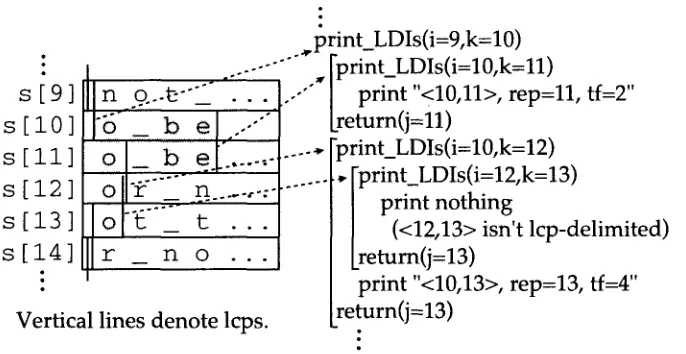
Figure 5 illustrates the function calls for c o m p u t i n g the nontrivial lcp-delimited intervals in Figure 4. C code is provided in A p p e n d i x A.Computational Linguistics Volume 27, Number 1
s [ 9
s[lO
s [ l l s [ 1 2
s [ 1 3 ] o " t ... t . . . s [ 1 4 ] r _ n o . . .
V e r t i c a l l i n e s d e n o t e lcps.
~.print L D I s ( i = 9 , k = 1 0 ) ... ~ [ p r i n t C D I s ( i = 1 0 , k = l l )
] n o . - ~ - " j _ . . . . ,-'" | p r i n t <10,11>, r e p = 1 1 , tf=2" ] "5~"" b e . , ' " ' " [return(j=11)
.... , " p r i n t _ L D I s ( i = 1 0 , k = 1 2 ) ] o _ b e. . . -, , [ p r i n t _ L D I s ( i = 1 2 , k = 1 3 ) ] o "±'"'---_.n ... -:- | p r i n t n o t h i n g ,
| (<12,13> i s n t l c p - d e l i m i t e d ) Lreturn(j=13)
p r i n t "<10,13>, r e p = 1 3 , tf=4" r e t u r n ( j - 1 3 )
Figure 5
Trace of function calls for computing the nontrivial lcp-delimited intervals in Figure 4. In this trace, trivial intervals are omitted. Print_LDIs(i = x,k = y) represents a function call with arguments, i and k. Indentation represents the nest of recursive calls. Print_LDIs(i,k) searches the right edge, j, of the non-trivial lcp-delimited interval, <i,j>, whose SIL is lcp[k]. Each representative, k, value is given to the function print_LDIs just once (dotted arcs).
p r i n t _ L D I s +- function(i, k) { j ~ k .
O u t p u t a trivial lcp-delimited interval <k, k> with tf = 1.
While lcp[k] <_ lcp~ + 1] and j + 1 < N, do j *-- print_LDIs(k, j + 1).
O u t p u t an interval <i,j> with tf = j - i + 1 and rep = k, if it is lcp-delimited. Return j. }
The second implementation (below) introduces its o w n explicit stack, a complica- tion that turns out to be important in practice, especially for large corpora. C code is p r o v i d e d in A p p e n d i x B.
p r i n t _ L D I s _ s t a c k *-- function(N){
stack_i ~-- an integer array for the stack of the left edges, i. stack_k ~ an integer array for the stack of the representatives, k. stack_i[O] *-- O.
stack_k[O] *-- O.
sp *--- 1 (a stack pointer). F o r j *-- 0,1,2 . . . N - 1 do
O u t p u t an lcp-delimited interval (j,j> with tf = 1. While Icp~ + 1] < lcp[stackd~[sp - 1]] do
O u t p u t an interval <i,j> with tf = j - i + 1, if it is lcp-delimited. s p * - - - s p - 1 .
stack_i[sp] ~-- stack_k[sp - 1]. stack_k [sp] *--- j + 1.
s p * - - - s p + l . }
[image:12.468.51.394.57.234.2]Yamamoto and Church Term Frequency and Document Frequency for All Substrings
Suffix A r r a y s[O] 2 I s[l] 15l s[2] !2_]
s[3] b I
s [4] 8 1
s [ 5 ] 181 - - - 4 s [ 6 ] 3 I s [ 7 ] 161 s [ 8 ] 4 i s [ 9 ] 17[
s [i0] 9 I
s[ll] s[12] 141 s[13] 6 1
s[14] 1--51
s[15] s[16] 111
s[iv] o--I
s[18] 1~1
Suffixes d e n o t e d by s [i] _ b e $ _ b e $ _ t o _ b e $
$
$
$
b e $ be$ e$ e$
n o t _ t o _ b e $ o _ b e $ o _ b e $ orS ot to b e $
r$
t _ t o _ b e $ t o _ b e $ t o _ b e $
D o c u m e n t id's icp[i] ofs[i]
0 0
4 2
I 2
0 0
I I
I 2
0 0
3 2
0 0
2 2
0 2
0 0
5 2
1 I
I 2
0 I
0 2
I 0
6 2
0 I n p u t d o c u m e n t s : dO = " t o _ b e $ " - -
d l = " o r S " d 2 = " n o t _ t o _ b e $ "
C o r p u s = dO + d l + d 2 = " t o _ b e $ o r $ n o t _ t o _ b e $ "
Resulting non-trivial lcp-delimited intervals: ('rep' m e a n s a representative, k.)
(0,1>, rep= 1, tf=2, df=2 (0, 2>, rep= 2, tf=3, df=2 (3, 5), rep= 4, tf=3, df=3 (6, 7>, rep= 7, tf=2, df=2 <8, 9/, rep= 9, tf=2, df=2 (11,12>, rep=12, tf=2, df=2 <11,14}, rep=13, tf=4, df=3 (17,18>, rep=18, tf=2, df=2 <16,18), rep=17, tf=3, dr=2
Figure 6
A suffix array for a corpus consisting of three documents. The special character $ denotes the end of a document. The procedure outputs a sequence of intervals with their term frequencies and document frequencies. These results are also presented for the nontrivial intervals.
2.6 Computing
df for All Classes
Thus far we have seen h o w to c o m p u t e term frequency, tf, for all substrings (n-grams) in a sequence (corpus). This section will extend the solution to compute d o c u m e n t frequency,
dr,
as well as term frequency. The solution runs inO(NlogN)
time a n dO(N)
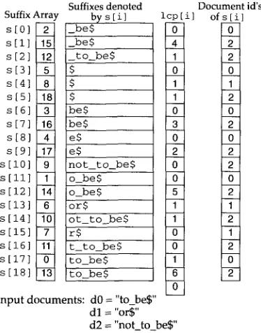
space. C code is p r o v i d e d in A p p e n d i x C.This section will use the r u n n i n g example s h o w n in Figure 6, where the corpus is: "to_be$or$not_to_be$'. The corpus consists of three documents, "to_be$', "orS", a n d
"not_to_be$'. The special character $ is used to denote the end of a document. The procedure outputs a sequence of intervals with their term frequencies a n d d o c u m e n t frequencies. These results are also presented for the nontrivial intervals.
The suffix array is c o m p u t e d using the same procedures discussed above. In ad- dition to the suffix array a n d the lcp vector, Figure 6 introduces a n e w third table that is used to m a p from suffixes to d o c u m e n t ids. This table of d o c u m e n t ids will be
[image:13.468.38.225.59.297.2]Computational Linguistics Volume 27, Number 1
used by the function get_docnum to map from suffixes to document ids. Suffixes are terminated in Figure 6 after the first end of document symbol, unlike before, where suffixes were terminated with the end of corpus symbol.
A straightforward method for computing d f for an interval is to enumerate the suffixes within the interval and then compute their document ids, remove duplicates, and return the number of distinct documents. Thus, for example, df("o') in Figure 6, can be computed by finding corresponding interval, (11,14}, where every suffix within the interval starts with "o" and no suffix outside the interval starts with "o'. Then we enumerate the suffixes within the interval {s[11],s[12],s[13],s[14]}, compute their document ids, {0, 2,1, 2}, and remove duplicates. In the end we discover that df("o") -- 3. That is, "o" appears in all three documents.
Unfortunately, this straightforward approach is almost certainly too slow. Some document ids will be computed multiple times, especially when suffixes appear in nested intervals. We take advantage of the nesting property of lcp-delimited intervals to compute all df's efficiently. The d f of an lcp-delimited interval can be computed recursively in terms of its constituents (nested subintervals), thus avoiding unnecessary recomputation.
The procedure print_LDIs_w±th_df presented below is similar to print_LDIs_- s t a c k but modified to compute d f as well as tf. The stack keeps track of i and k, as before, but n o w the stack also keeps track of df.
i, the left edge of an interval, k, the representative (SIL = lcp[k]),
df, partial results for dr, counting documents seen thus far, minus duplicates. print_LDIs with_dr +--- function(N){
stack_i ~- an integer array for the stack of the left edges, i. stack_k ~ an integer array for the stack of the representatives, k. s t a c k d f ~-- an integer array for the stack of the df counter.
doclink[O..D] : an integer array for the document link initialized with - 1 . D = the number of documents.
stack_i[O] ~ O. stack_k[O] *--- O. stack_dr[O] *--- 1.
sp ~ 1 (a stack pointer). (1) F o r j ~ 0 , 1 , 2 , . . . , N - 1 do
(2) (Output a trivial lcp-delimited interval q,j> with tf = 1 and d / = 1.) (3) doc *-- get_docnum(s~])
(4) if doclink[doc] ~ - 1 , do
(5) let x be the largest x such that doclink[doc] >_ stack_i N . (6) stack_dr[x] *--- stack_df[x] - 1.
(7) doclink[ doc] ~-- j. (8) d f ,-- 1.
(9) While lcp~" + 1] < lcp[stack_k[sp - 1]] do (10) d f *--- stack~tf[sp - 1] + d f .
(11) Output a nontrivial interval (i,j) with tf = j - i + 1 and dr, if it is lcp-delimited.
(12) sp ~-- sp - 1.
(13) stack_i[sp] ~-- stack_k[sp - 1]. (14) stack_k [sp] ~-- j + 1.
Yamamoto and Church Term Frequency and Document Frequency for All Substrings
(15) staek_e/[sp] ~ ad. (16) sp *-- sp + 1. }
Lines 5 and 6 take care of duplicate documents. The duplication processing makes use of
doclink
(an array of length D, the number of documents in the collection), which keeps track of which suffixes have been seen in which document,doclink
is initialized with - 1 indicating that no suffixes have been seen yet. As suffixes are processed,doclink
is updated (on line 7) so that
doclink
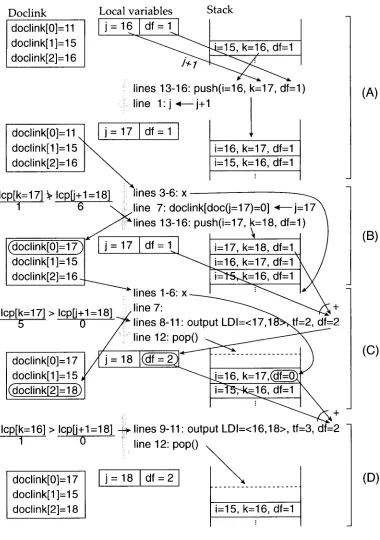
[d] contains the most recently processed suffix in document d. As illustrated in Figure 7, when j = 16 (snapshot A), the most recently processed suffix in document 0 is s[11] ("o_be$"), the most recently processed suffix in document 1 is s[15] ("r$"), and the most recently processed suffix in document 2 is s[16] ("t_to_be$"). Thus, doclink[0]= 11, doclink[1]= 15, and doclink[2]= 16. After processing s[17] ("to_be$"), which is in document 0, doclink[0] is updated from 11 to 17, as shown in snapshot B of Figure 7.Stackdf
keeps track of document frequencies as suffixes are processed. The invari-ant is:
stack_dr[x]
contains the document frequency for suffixes seen thus far starting at i =stack_i[x]. (x
is a stack offset.) When a new suffix is processed, line 5 checks for double counting by searching for intervals on the stack (still being processed) that have suffixes in the same document as the current suffix. If there is any double counting,stackdf
is decremented appropriately on line 6.There is an example of this decrementing in snapshot C of Figure 7, highlighted by the circle around the binding of
df
to 0 on the stack element: [i = 0, k = 17,df
= 0]. Note thatdf
was previously bound to 1 in snapshot B. The binding ofdf
was decremented when processing s[18] because s[18] is in the same document as s[16]. This duplication was identified by line 5. The decrementing was performed by line 6. Intervals are processed in depth-first order, so that more deeply nested intervals are processed before less deeply nested intervals. In this way, double counting is only an issue for intervals higher on the stack. The most deeply nested intervals are trivial intervals. They are processed first. They have adf
of 1 (line 8). For the remaining nontrivial intervals,staekdf
contains the partial results for intervals in process. As the stack is popped, thedf
values are aggregated up to compute thedf
value for the outer intervals. The aggregation occurs on line 10 and the popping of the stack occurs on line 12. The aggregation step is illustrated in snapshots C and D of Figure 7 by the two ar- rows with the " + " combination symbol pointing at a value ofdf
in an output statement.2.7 Class Arrays
The classes identified by the previous calculation are stored in a data structure we call a class array, to make it relatively easy to look up the term frequency and document frequency for an arbitrary substring. The class array is a stored list of five-tuples:
(SIL,
LBL, tf, df, longest suffix I. The
fifth element of the five-tuple is a canonical member ofthe class (the longest suffix). The five-tuples are sorted by the alphabetical order of the canonical members. In our C code implementation, classes are represented by five integers, one for each element in the five-tuple. Since there are N trivial classes and at most N - 1 nontrivial classes, the class array will require at most 10N - 5 integers. However, for many practical applications, the trivial classes can be omitted.
Figure 8 shows an example of the nontrivial class array for the corpus: "to_be$or$ not_to_be$". The class array makes it relatively easy to determine that the substring "o" appears in all three documents. That is, df("o") = 3. We use a binary search to find that tuple c[5] is the relevant five-tuple for "o". Having found the relevant tuple, it requires a simple record access to return the document frequency field.
Computational Linguistics Volume 27, N u m b e r 1
Doclink
doclink[0]=11
doclink[1]=15
doclink[2]=16
Local variables
Stack
I j = 1 6
df:Ll' I
I
lines 13-16: push(i=16, k=l 7, df=l )
line l : j ~ j + l
doclink[0]=114 J =17 df=l
doclink[1]=15 I ~
i=16, k=17, df=l
doclink[_2]--16 I ~
i=15, k=16, df=l
\
lop[k=17] ~. Icp[j+1=18]
lines 3-6: x
1
6
~ l i n e
7: doclink[doc(j=17)=0] . ~ j = 1 7 ~
~ l i n e s
13-16:push(i=17, k=l 8, df=l )
J:'7 df:\Li=17, k:18, df=1, l)
doclink[1]=15/
"'--.~=16, k=17, df=l~ /
doclink[2]=16.J..._~
I
df=l l Y
linesl-6:x__l
~ I J \ + -I c p [ k = 1 7 ]
> Icp[j+1=18] _/line 7:
~
"
'
"
~
5
0
~
lines 8-11: output LDI--<17,18~=2~=2
/ "
line12:pap0 ~
~
~
~
~ 7 - - - ~ / / ] v j :
18 ~ ~ - -
l .... : ... --- )
doclink[1]= 15 dt /
-'----~-.=16, k= 17,(.df=O.), "
~doclink[2]=18)l
l i - - ~ ,
df=l
\
Icp[k=16] > Icp[j+1=18] ~ lines 9-11" output LD1=<16,18>, tf=3, df=2
-1 0 '
line 12: pop()
I j = 1 8 df=2
. ... ...
doclink[0]=17
doclink[1 ]=15
doclink[2]=l 8
i=15, k=16, df=l
(A)
(B)
(c)
(D)
Figure 7
Snapshots of the doclink array and the stack during the processing of print_LDIs_with_df on the corpus: "to_be$or$not_to_be$'. The four snapshots A - D illustrate the state as j progresses from 16 to 18. Two nontrivial intervals are emitted while j is in this range: (17,18) and (16,18). The more deeply nested interval is emitted before the less deeply nested interval.
[image:16.468.53.433.61.601.2]Yamamoto and Church Term Frequency and Document Frequency for All Substrings
Class array The longest suffix (Pointer to cor ~us) denoted by c[i] SIL
c [ 0 ]
0
_
1
c [i]
0
_ b e $
4
c [ 2 ] 5 $ 1
c
[3]
3be$
3c
[4]
4e$
2c [ 5 ]
1
o
1
c
[6]
1
o_be$
5
c[7]
11t
1 [image:17.468.37.284.59.235.2]c [ 8 ]
0
t o _ b e $
6
Figure 8An example of the class array for the cor
LBL tf df
0
3
2
1
2
2
0
3
3
0
2
2
0
2
2
0
4
3
1
2
2
0
3
2
1
2
2
pus: "to _be$or$not_to_be$".
3. Experimental Results
3.1 RIDF and MI for English and Japanese
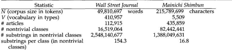
We used the methods described above to compute dr, tf, and RIDF for all substrings in two corpora of newspapers summarized in Table 1. MI was computed for the longest substring in each class. The entire computation took a few hours on a MIPS10000 with 16 Gbytes of main memory. The processing time was dominated by the calculation of the suffix array.
The English collection consists of 50 million words (113 thousand articles) of the Wall Street Journal (distributed by the ACL/DCI) and the Japanese collection consists of 216 million characters (436 thousand articles) of the CD-Mainichi Shimbun from 1991- 1995 (which are distributed in CD-ROM format). The English corpus was tokenized into words delimited by white space, whereas the Japanese corpus was tokenized into characters (typically two bytes each).
[image:17.468.35.416.583.666.2]Table I indicates that there are a large number of nontrivial classes in both corpora. The English corpus has more substrings per nontrivial class than the Japanese corpus. It has been noted elsewhere that the English corpus contains quite a few duplicated articles (Paul and Baker 1992). The duplicated articles could explain w h y there are so m a n y substrings per nontrivial class in the English corpus when compared with the Japanese corpus.
Table 1
Statistics of the English and Japanese corpora.
Statistic Wall Street Journal Mainichi Shimbun
N (corpus size in tokens) V (vocabulary in types) # articles
# nontrivial classes
# substrings in nontrivial classes substrings per class (in nontrivial
classes)
49,810,697 words 215,789,699 characters
410,957 5,509
112,915 435,859
16,519,064 82,442,441
2,548,140,677 1,388,049,631
154.3 16.8
Computational Linguistics Volume 27, Number 1
25
20
15
[ ~ 1 0
5
0
-5
-10
5f, I
ll..
. . . __, , . - . , _ - . . . .i1:
. . . . , ~ - - 1 5 --20 2 5 3'0 35 40 f - - - 5 . . . . ,(f 15 20 25 3() 35 40• . L e n g t h -,
Length
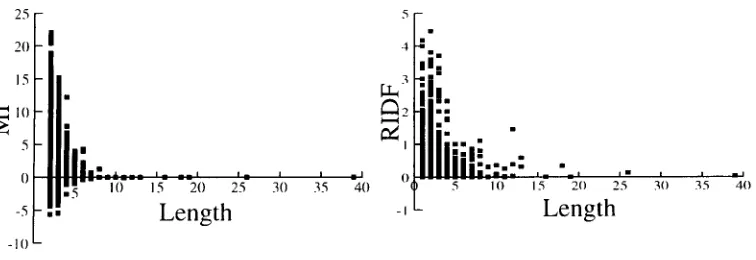
Figure 9
The left panel plots MI as a function of the length of the n-gram; the right panel plots RIDF as a function of the length of the n-gram. Both panels were computed from the Japanese corpus. Note that while there is more dynamic range for shorter n-grams than for longer n-grams, there is plenty of dynamic range for n-grams well beyond bigrams and trigrams.
For subsequent processing, we excluded substrings with tf < 10 to avoid noise, resulting in about 1.4 million classes (1.6 million substrings) for English and 10 million classes (15 million substrings) for Japanese. We computed RIDF and MI values for the longest substring in each of these 1.4 million English classes and 10 million Japanese classes. These values can be applied to the other substrings in these classes for RIDF, but not for MI. (As mentioned above, two substrings in the same class need not have the same MI value.)
MI of each longest substring, t, is computed by the following formula.
M I ( t = x Y z ) = log p ( z y ) p ( z l y ) p ( x v z ) q(~Yz)
N
l°r:, q(xY) q(Yz) N q(Y) ff(~g~)ff(Y) = log t f ( x Y ) t f ( Y z ) "
where x and z are tokens, and Y and z Y z are n-grams (sequences of tokens). When Y is the empty string, tf(Y) -- N.
Figure 9 plots RIDF and MI values of 5,000 substrings randomly selected as a func- tion of string length. In both cases, shorter substrings have more dynamic range. That is, RIDF and MI vary more for bigrams than million-grams. But there is considerable dynamic range for n-grams well beyond bigrams and trigrams.
3.2 Little C o r r e l a t i o n b e t w e e n R I D F a n d M I
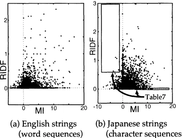
We are interested in comparing and contrasting RIDF and MI. Figure 10 shows that RIDF and MI are largely independent. There is little if any correlation between the RIDF of a string and the MI of the same string. Panel (a) compares RIDF and MI for a sample of English word sequences from the WSJ corpus (excluding unigrams); panel (b) makes the same comparison but for Japanese phrases identified as keywords on the CD-ROM. In both cases, there are many substrings with a large RIDF value and a small MI, and vice versa.
[image:18.468.55.433.56.186.2] [image:18.468.166.323.393.482.2]Yamamoto and Church Term Frequency and Document Frequency for All Substrings
2
1
2 'i° ~
: , • ~ .~ :
a
..,"
~, • ~ ¥" * .
i • •
' • # • • • • 1
• • • • • •
; ' . ' . - • • l L - - M . •
l , % , ; •
. . . . ' : " . . . 0 -~::
i i i
0 M I fo 2o -10 0 MI 10 20
(a) English strings
(word sequences)
(b) Japanese strings
(character sequences)
F i g u r e 10
Both panels plot RIDF versus MI. Panel (a) plots RIDF and MI for a sample of English n-grams; panel (b) plots RIDF and MI for Japanese phrases identified as keywords on the CD-ROM. The right panel highlights the 10% highest RIDF and 10% lowest MI with a box, as well as the 10% lowest RIDF and the 10% highest MI. Arrows point to the boxes for clarity.
We believe the t w o statistics are b o t h useful b u t in different w a y s . Both p i c k o u t interesting n - g r a m s , b u t n - g r a m s w i t h large MI are interesting in different w a y s f r o m n - g r a m s w i t h large RIDF. C o n s i d e r the English w o r d s e q u e n c e s in Table 2, w h i c h all contain the w o r d
having.
These sequences h a v e large MI v a l u e s a n d small RIDF values. In o u r collaboration w i t h lexicographers, especially those w o r k i n g o n dictionaries for learners, w e h a v e f o u n d considerable interest in statistics such as MI that pick o u t these k i n d s of phrases. Collocations can be quite challenging for n o n n a t i v e s p e a k e r s of the language. O n the other h a n d , these k i n d s of p h r a s e s are n o t v e r y g o o d k e y w o r d s for i n f o r m a t i o n retrieval.T a b l e 2
English word sequences containing the word
having.
Note that these phrases have large MI and low RIDF. They tend to be more interesting for lexicography than information retrieval. The table is sorted by MI.tf df RIDF MI Phrase
18 18 -0.0 10.5 admits to having 14 14 -0.0 9.7 admit to having 25 23 0.1 8.9 diagnosed as having 20 20 -0.0 7.4 suspected of having 301 293 0.0 7.3 without having
15 13 0.2 7.0 denies having 59 59 -0.0 6.8 avoid having 18 18 -0.0 6.0 without ever having 12 12 -0.0 5.9 Besides having 26 26 -0.0 5.8 denied having
[image:19.468.37.332.60.285.2] [image:19.468.38.243.561.673.2]Computational Linguistics Volume 27, Number 1
Table 3
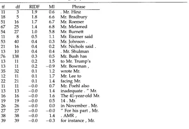
English word sequences containing the word Mr. (sorted by RIDF). The word sequences near the top of the list are better keywords than the sequences near the bottom of the list. None of them are of much interest to lexicography.
tf df RIDF MI Phrase
11 3 1.9 0.6 . Mr. Hinz
18 5 1.8 6.6 Mr. Bradbury
51 16 1.7 6.7 Mr. Roemer
67 25 1.4 6.8 Mr. Melamed
54 27 1.0 5.8 Mr. Burnett
11 8 0.5 1.1 Mr. Eiszner said
53 40 0.4 0.3 Mr. Johnson.
21 16 0.4 0.2 Mr. Nichols said.
13 10 0.4 0.4 . Mr. Shulman
176 138 0.3 0.5 Mr. Bush has
13 11 0.2 1.5 to Mr. Trump's
13 11 0.2 -0.9 Mr. B o w m a n ,
35 32 0.1 1.2 wrote Mr.
12 11 0.1 1.7 Mr. Lee to
22 21 0.1 1.4 facing Mr.
11 11 -0.0 0.7 Mr. Poehl also 13 13 -0.0 1.4 inadequate. " Mr. 16 16 -0.0 1.6 The 41-year-old Mr.
19 19 -0.0 0.5 14. Mr.
26 26 -0.0 0.0 in N o v e m b e r . Mr. 27 27 -0.0 -0.0 " For his p a r t , Mr. 38 38 -0.0 1.4 . A M R ,
39 39 -0.0 -0.3 for instance, Mr.
Table 3 s h o w s M I a n d RIDF v a l u e s for a s a m p l e of w o r d s e q u e n c e s c o n t a i n i n g the w o r d Mr. The table is s o r t e d b y R I D E The s e q u e n c e s n e a r the t o p of the list are better k e y w o r d s t h a n the s e q u e n c e s f u r t h e r d o w n . N o n e of these s e q u e n c e s w o u l d b e of m u c h interest to a l e x i c o g r a p h e r (unless he or she w e r e s t u d y i n g n a m e s ) . M a n y of the s e q u e n c e s h a v e r a t h e r small MI values.
Table 4 s h o w s a f e w w o r d s e q u e n c e s starting w i t h the w o r d the w i t h large M I values. All of these s e q u e n c e s h a v e h i g h MI (by construction), b u t s o m e are h i g h in RIDF as well (labeled B), a n d s o m e are n o t (labeled A). M o s t of the s e q u e n c e s are interesting in o n e w a y or another, b u t the A s e q u e n c e s are different f r o m the B sequences. The A s e q u e n c e s w o u l d be of m o r e interest to s o m e o n e s t u d y i n g the g r a m m a r in the WSJ s u b d o m a i n , w h e r e a s the B s e q u e n c e s w o u l d b e of m o r e interest to s o m e o n e s t u d y i n g the t e r m i n o l o g y in this s u b d o m a i n . The B s e q u e n c e s in Table 4 t e n d to pick o u t specific e v e n t s in the n e w s , if n o t specific stories. T h e p h r a s e , the Basic Law, for e x a m p l e , picks o u t a p a i r of stories that discuss the e v e n t of the h a n d o v e r of H o n g K o n g to China, as illustrated in the c o n c o r d a n c e s h o w n in Table 5.
Table 6 s h o w s a n u m b e r of w o r d s e q u e n c e s w i t h h i g h M I containing c o m m o n prepositions. The h i g h MI indicates a n interesting association, b u t a g a i n m o s t h a v e l o w RIDF a n d are n o t p a r t i c u l a r l y g o o d k e y w o r d s , t h o u g h there are a f e w e x c e p t i o n s (Just for Men, a w e l l - k n o w n b r a n d n a m e , h a s a h i g h RIDF a n d is a g o o d k e y w o r d ) .
T h e J a p a n e s e s u b s t r i n g s are similar to the English substrings. Substrings w i t h h i g h RIDF p i c k o u t specific d o c u m e n t s ( a n d / o r events) a n d therefore t e n d to b e relatively g o o d k e y w o r d s . Substrings w i t h h i g h M I h a v e n o n i n d e p e n d e n t distributions (if n o t n o n c o m p o s i t i o n a l semantics), a n d are therefore likely to b e interesting to a lexicogra- p h e r or linguist. Substrings that are h i g h in b o t h are m o r e likely to b e m e a n i n g f u l units
[image:20.468.52.436.110.372.2]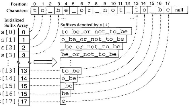
![Figure 4 Six suffixes are copied from Figure 3, s[9]-s[14], along with eight of their lcp-delimited intervals](https://thumb-us.123doks.com/thumbv2/123dok_us/1273111.655396/8.468.53.361.56.358/figure-suffixes-copied-figure-s-lcp-delimited-intervals.webp)