Bandwidth Assignment in a Cluster-based Wireless
Sensor Network
Tarek Azizi, Rachid Beghdad, Mourad Oussalah
Abstract—Wireless sensor networks (WSN) are constrained by the processing speed, storage capacity, collision avoidance and energy which they are fundamental aspects in the development of communication protocols, and in this context, most research projects in this area focus on the aspect of energy, and ignore some QoS supports also interesting and unexplored, such as bandwidth, response time, ... Sensor networks require features such as energy conservation, the ability of scalability, fault tolerance and adaptability to topology changes. Indirectly, a communications protocol that avoids collisions saves energy, since the need to retransmit a message is reduced. The access to the communication medium by time-division multiplexing (TDMA) is a reasonable technique to avoid collisions.
This paper mainly focuses on improving Masri’s [1] TDMA protocol in tree-based clustered wireless sensor network, where the density of the network at the user level is translated by the bandwidth at the network. We prove firstly that the used formulas in [1] is false, after that, simulations results prove the robustness of our formulas and show that our approach outperforms Masri’s one.
Index Terms—Wireless Sensor Networks, TDMA, QoS, Synchronization, Bandwidth.
I.INTRODUCTION
Advanced technologies in the field of computer networks have enabled the development of vast and various fields of applications. This diversity has brought computer networks support different traffic types and provide services that must be both a generic and adaptive applications since the properties of quality of service (QoS) are different from application type to another. For example, real-time multimedia applications require very minimal transfer times; guaranteed bandwidth and low packet loss, while applications of wireless sensor networks (WSN) are mainly solve the management problem of the energy consumption. However, these two types of applications are facing the problem of scaling. In this context, the hierarchical routing based on the clustering imposes as a very promising approach to solve this problem [1].
In fact, we can view the support of QoS in WSNs from different perspectives according of the layered architecture of distributed systems [1], so it might be considered from the user point of view as the precision, density, the accuracy or the lifetime, thus as bandwidth, delay jitter the point of view of the network. Because of these different views of service quality, it is essential to find the relationships
Manuscript received March 23rd 2013; accepted April 3rd 2013. Tarek Azizi, is with the Faculty of Sciences, Abderrahmane MIRA University, Bejaïa, Algeria, ([email protected])
Rachid Beghdad, is within Faculty of Sciences, Abderrahmane MIRA University, Bejaïa, Algeria., ([email protected])
Mourad Oussalah is with University of Birmingham, Electronics, Electrical and Computer Engineering Edgbaston, Birmingham,
B15 2TT, UK, ([email protected])
between these different QoS requirements on different levels, to achieve a coherent system. Once the relationship between these parameters is found, they could correctly translate from each level to another one (QoS mapping process).
In this paper, we prove prove first that the used formulas in [1] is false. Second, we propose new formulas and show the relationship between different parameters of QoS (as density at user level QoS and bandwidth reserved for each sensor at network level QoS). We prove the strong coupling between the two parameters of a WSN by calculating the length of a TDMA superframe according to the depth of the tree in clusters. To validate our theoretical results, we present simulations that demonstrate the relationship between QoS parameters mentioned above.
In section 2, we present some related works about QoS support in WSN. In Section 3, we present some requirements of bandwidth allocation in WSN using TDMA. After that, Masri’s approach [1] is described in section 4. In the same section, we present our work that consists to calculate the length of TDMA superframe according to network density, and we show how to translate the QoS parameter (density) level user, to a QoS parameter (bandwidth) network level. In Section 5, we present our simulations that confirm our formulas presented in Section 5 and we discuss the relationship between density and bandwidth with other parameters. We conclude our paper in Section 6 by a conclusion and perspectives.
II. RELATED WORK
and this translation is achieved when identifying the position of the lost packets on the data flow and computing the effect
of those lost packets on the frames sent by the
source (we can seen this impact on the application layer). In WSN, there is a limited works done on the derivation of QoS which, the most, covers agreements between QoS parameters such as energy, density, latency, accuracy ... etc. The network QoS performance characteristic for the loss parameter is mapped from lower to upper layer in a quantifiable way. In [8], a formal methodology is presented to translate application level SLA "Service Level Agreement" (response time) to network performance (link bandwidth and router throughput). Authors provides a statistical analysis on mapping application level’s response time to network related parameters such as link bandwidth and router throughput by using some simple queuing models. In [9], simulations of the QoS parameters in a WSN have been done to better understanding the tradeoffs between density, latency and accuracy. The authors also explored the trade-off between density and energy, and study the effect of infrastructure decisions on the performance of a sensor network. They show the performance both in terms of network efficiency as well as meeting the application accuracy and latency demands. In [10], QoS is defined as the optimum number of sensors that should be sending information at any given time (because sensor deaths and sensor replenishments make it difficult to specify this number) by using the idea of allowing the base station to communicate QoS information to each of the sensors using a broadcast channel and using the mathematical paradigm of the Gur Game to dynamically adjust to the optimum number of sensors.
III. TDMA PROTOCOL IN WSN
In TDMA protocol, nodes share the available bandwidth in time as “bandwidth sharing method”. The available bandwidth is divided on the frame [13], where each frame is divided into time slots. On the other hand, energy and fast and efficient query response is another issue of WSN
[16]. From these characteristics which are depicted above, our proposed TDMA protocol must be energy efficient. Since collision does not occur in TDMA protocols, data retransmission is avoided.
To design an efficient TDMA protocol for wireless sensor network the following attributes must be considered [17]: - Energy Efficiency: it is often very difficult to change or recharge batteries for the sensors. Sometimes it is beneficial to replace the sensor node rather than recharging them. - Scalability and adaptability to change: any change in network size, node density and topology, should be handled effectively by TDMA protocols.
- Latency: the detected events in WSN applications must be reported to the sink in real time for an immediate appropriate response action.
- Fairness: it is important to guarantee that the sink node receives information from all sensor nodes fairly when bandwidth is limited in many WSN applications.
There are other attributes such as throughput and bandwidth utilization. In TDMA Based MAC protocol, network is assumed to be formed as clusters. Each one of these clusters is managed by a Cluster Head (CH). The CH collects the information from his child nodes within its cluster, carries data merging, communicates with the other CHs and finally sends the data to the sink. This CH performs the assignment of the time slots to his child nodes [17].
IV. EXPERIMENTAL METHODOLOGIES
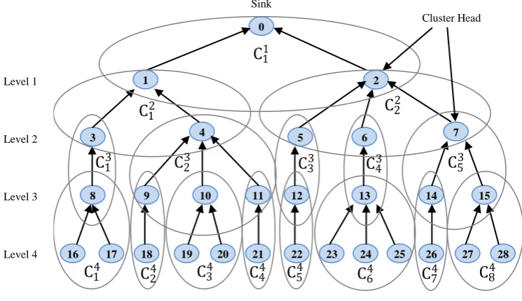
[image:2.595.110.483.490.705.2]To compute the length of our TDMA superframe and to understand the relationship between the density changes and the bandwidth reserved for each node, we illustrated in Figure 1 an example of running TDMA without collisions in a tree-based WSN.
Fig. 1. Tree-based clustered Sensor network
The problem here is: how to run TDMA by the nodes of different levels without any collision ? For example, nodes 3, 5, 18, 19, 21, 25, 26, and 27 can run simultanuously TDMA, and so on …
0
1 2
3 4
8
16 17
9 10 11
18 19 20 21
5 6 7
12
22 23 24 25 13
26 14
27 28 15
Sink
Cluster Head
Level 1
Level 2
Level 3
Level 4
C
11C
12C
22C
13C
2
3
C
33
C
43C
53C
14C
A. Assumptions and working environment
We consider a sensor network based on assumptions concerning the type of network considered and the synchronization of nodes, where these characteristics are:
a) Network type: Since a sensor network consists of nodes randomly deployed according to an architecture, we assume that our network architecture is hierarchical “tree-based”, and that the sensors are grouped into clusters, which inter-cluster communications are done by Clusters Head (CHs).
b) Synchronization of sensors: The time synchronization of the network can be carried out by applying a synchronization algorithm [11], or by sending a signal from the sinks or other entity capable of reaching all sensors [12].
The synchronization range defines the nodes in the network that are required to be synchronized. Depending on the application, the range includes all or only a subset of nodes. Synchronization triggered by an event (Event-triggered synchronization) may be limited to the subset of nodes collocated who observe the event in question [11].
B. Superframe length computation a) Notations
To determine the superframe length of the proposed approach that will be generated, we need some notations, (which are inspired from [1]):
- 𝐶𝑖ℎ: denotes the cluster number i at level h.
- CH(x) return the CH of cluster x, while CH−1(x) return the cluster which has x as CH.
- S(x) is a boolean is equal to 1 if child nodes in cluster x sense data and 0 otherwise.
- Ch(x) return number of all child nodes in cluster x. - Nc(h) return the number of clusters at level h.
Nc h =
1 If h = 1 Ch Cih−1
Nc h−1
i=1 If h ≠ 1
1
- L(x) returns the number of leaf nodes whose ancestor is the CH of cluster x, where H means the tree depth:
L Cih =
Ch Cih If h = H L Cjh+1 Ch Ckh
i k=1
j= i−1k=1 Ch Ckh +1 If h ≠ H
2
- Ns(x) returns the number of all sensing child nodes whose ancestor is the CH of cluster x (with Ns(0) = 0).
Ns Cih =
Ch Cih h = H S Cih × Ch Cih +
L Cjh+1 Ch Ckh
i k=1
j= i−1 Ch Ckh +1 k=1
If h ≠ H
3
b) Superframe length according to MASRI W. and Mammeri Z. [1]
In order to calculate the length of superframe and to determine the bandwidth reserved for each sensor (node) and after a series of experiments, W. Masri and Z. Mammeri [1] proposed a formula (4) to calculate the total length of the superframe (fig. 2) presented as follows:
Length = Maxi=1Nc 1 Ns Ci1 + Maxi=1Nc 2 Ns Ci2 if L Cih ≤ Maxj=1Nc h−2 L Cjh−2 − L F(Cih) ∀ Cih, i ∈ 1, Nc h , h ∈ 3, H 4
c) Critics
We can see from this formula that there are some nodes that can transmit data at the same time (like nodes 5, 6 and with node 1, and nodes 3 and 4 with sensor 2 for example). So, this will lead to collisions and we can conclude that this formula is FALSE (!)
d) Process and proposed approaches
In order to increase the bandwidth reserved for each node sensor and to limit the problem of collisions among sensors, we propose a communication architecture where nodes communicate using TDMA, and to do so, we proposed a formula (formula 5) which allows us to calculate the superframe length (fig. 3) where the sensing of events is done by all nodes and simultaneous transmissions are performed by the same level clusters as well as remote nodes of 3 hops. In all cases above, the intermediate nodes also sense and transmit data. In this case, we should add the number of time slots required for intermediate nodes to send their own flows. This formula is based on the notations in [1].
C. Proposed formula
In the following we will introduce our formula (5) to improve the Masri’s one [1], which is better than the last one in terms of bandwidth allocation.
Length
= Maxi=1Nc 2 Ns Ci2 + 1
+ Maxi=1Nc 2 Maxi=1Nc 2 Ns Ci2 ; Maxi=1Nc 1 Ns Ci1
− Maxi=1Nc 2 Ns Ci2 + 1
+ Maxi=1Nc 3 Ns Ci3 ∀ Cih, i ∈ 1, Nc h , h ∈ 1, H (5)
Our formula (5) avoids collisions caused by simultaneous transmissions of nodes in the same cluster in one hand, and allows much more sensors to communicate with each other in each slot time on the other hand.
D. Metrics to be evaluated
To evaluate network performances we are interested in following quality of services metrics:
- Superframe length: it is the period where all sensor nodes of the network transmit there frames to the base station, so they are ready to transmit again (Round).
- Bandwidth: the amount of traffic sent by each node in the network during the simulation time. This metric varies along the length of superframe calculated according to the network density. This bandwidth is calculated by formula (6):
B n = Ns CH
−1 n + 1
Length 6
- Stream capacity: it is the sum of all traffic sent by a node and received by the base station during the simulation. This metric allows studying the problem of appropriate sharing of bandwidth between nodes.
We will now compare our approach to Masri’s one by illustrating them in the following figures (Fig. 2 and Fig. 3) From formula (4), the superframe length is composed of two parts which are (Fig. 2):
Maxi=1Nc 1 Ns Ci1 : represents the sum total of all sensor
nodes in the network (which gives to us 28 slots time),
Maxi=1Nc 2 Ns Ci2 : represents the maximum number of all
child nodes that do sensing whose ancestor is between child nodes of level 1. (In this case, the sensor CH1 has 12 time slots and the sensor CH2 has 14 time slots, then
[image:4.595.75.506.174.510.2]Maxi=1Nc 2 Ns Ci2 =14).
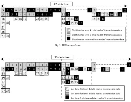
Fig. 2. TDMA superframe
Fig. 3. Reduced TDMA superframe
Figure 3 shows that, from formula (5), the superframe length is composed of three parts which are:
Maxi=1Nc 2 Ns Ci2 + 1 : represents the maximum number of
all child nodes that do sensing whose ancestor is between the child nodes of level 1 plus one for the sensor itself,
Maxi=1Nc 2 Maxi=1Nc 2 Ns Ci2 ; Maxi=1Nc 1 Ns Ci1 − Maxi=1Nc 2 Ns Ci2 + 1 : is the maximum between the
number calculated by 𝑀𝑎𝑥𝑖=1𝑁𝑐 2 𝑁𝑠 𝐶𝑖2 + 1, and the sum of all child nodes that are do sensing whose ancestors is child nodes of level 1 except those cited by the last formula. In addition, there is no collision here.
We can conclude from these figures that our approach provides a reduced size of superframe length regardless of the network relatively to that proposed in [1].
V. PERFORMANCE STUDY
Using OMNeT Simulator, we have conducted several simulations to prove our formulas proposed for guaranteeing bandwidth, with the following settings:
TABLEI SIMULATION PARAMETERS
Number of sensors 28
Packets size 90 Octets
Simulation duration 150 s
MAC layer TDMA
Channel bit rate 9.6 Kbps Length of Slot time 75 ms
A. Bandwidth allocation
In Figure 4, we compares the results obtained using our superframe calculated by the formula described in [2] and the formula of our approach, where the cluster C34 has two
child nodes, i.e. Chinit 𝐶34 = 2 and MCh 𝐶34 = 6 (calculated using the formula (10) in [2]).
In this simulation, we increase the number of child nodes in this cluster gradually until reaching the MCh, for Ch 𝐶34 = 3, 4, 5, 6, and then exceeding for Ch 𝐶34 = 7 8, 9, 10, 11. Note that in this case the bandwidth decreases gradually 25
24 23 17
16 22
28 27 26 21
20 19 18
15
15 15
14
14
13
13 13 13
12
12 9 9 10 10 10 11 11
8
8 8
4 4 4 4
4 4 4 4
3 3
7 7 7
7 7 7
6 6
6 6 6
5
5 5 1 1 2 2
3 3
42 slots time
Slot time for level 4 child nodes’ transmission data
Slot time for level 3 child nodes’ transmission data
Slot time for Intermediates nodes’ transmission data
1 1 1 1 1 1 1 1 1 1 1 1 1 2 2
5
5 5 6 6 6 6 6 7 7 7 7 7 7 3 3 4 4
8 8 8
9 9 10 10 10 11 12 12
13 13 13 13
14 14 15 15 15
18 19 20 21 26 27 28
22 16 17 23 24 25
36 slots time
Slot time for level 4 child nodes’ transmission data
Slot time for level 3 child nodes’ transmission data
Slot time for Intermediates nodes’ transmission data
when adding other nodes, then it begins to decline more rapidly when it exceeds MCh.
Fig. 4. Relationship between network density and bandwidth
According to Figure 4, our approach provides better bandwidth because, and from the formula (6), the length of superframe is the denominator of bandwidth rate, so if we reduce the superframe length (as in the case of our approach compared with that described in [1]), the rate will increase, and vice versa (inverse relationship). We may conclude that, practically, this means that adding another node in the network, increase the superframe length and thus reduce the reserved bandwidth for each one. B. Relationship between superframe length, the reporting
period and the packet size
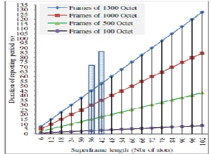
[image:5.595.69.275.516.666.2]From Figure 5, the duration of reporting periodic is directly related to the superframe length and it also depends on the packet size. In this case, changing of one parameter could affect others. For example, to increase the data freshness (i.e. decrease the duration of the reporting period), the length of the superframe should be reduced either by removing time slots (i.e. minimizes the number of nodes), or reducing the size of packets allowed to be sent by each node. In both cases, the accuracy will be adversely affected. So there is clearly a tradeoff between these parameters.
Fig. 5. Relationship between the superframe length, the reporting period and the packet size
Figure 5 shows how the reporting period increases when the density of the network increases, due to the superframe length.
We may also notice that the nodes allowed to send packets of large sizes (e.g. 1500 bytes) in their time slots, are always more affected by increasing the superframe length. In a WSN with 28 nodes deployed, allowing each one to send a
packet of 1500 Bytes in its time slot, the duration of reporting period (or data freshness) reaches 45 seconds (52.5 seconds with superframe depicted in [1]), and the same thing where each node is allowed to send a packet of 1000, 500 and 100 Bytes, the duration of reporting period reaches 29.88, 15.12 and 2.98 seconds respectively (34.86, 17.64 and 3.48 seconds with superframe calculated in [1]).
VI. CONCLUSION
The QoS support is one of the least explored aspects in the WSNs field despite its importance for many necessary types of applications (e.g. real-time applications). In this paper, we discuss an approach for the derivation of user-level QoS parameter (density) at network level QoS parameters (bandwidth), while calculating the TDMA superframe length, and presenting the bandwidth depending on the superframe length and the density of the network.
The only source of energy for sensor nodes is usually provided by batteries that have a limited life. To optimize energy consumption, nodes are organized into sets of active sensors that provide connectivity knowing that one set will be active at any time.
Once we calculated the superframe length, we establish the relationship between this length for a given topology, expressed, on one hand, in terms of density, and the bandwidth in the other. We calculated the rate of bandwidth, and we showed how the position of the added node has a direct impact on the length of superframe and hence on the allocated bandwidth.
REFERENCES
[1] Wassim Masri, Zoubir Mammeri. « Mapping density to bandwidth in tree-based wireless sensor networks », 43: 73–81, DOI 10.1007/s11235-009-9194-5, Telecommun Syst (2010).
[1] Omar Moussaoui : « Routage hiérarchique basé sur le clustering : garantie de QoS pour les applications multicast et réseaux de capteurs », [S.l.] : [s.n.], 2006. Université de Cergy-Pontoise: (2006). [3] Masri, W., & Mammeri, Z. « On QoS mapping in TDMA based
wireless sensor networks ». In IFIP international conference on personal wireless communications (pp. 329–342), (2008).
[4] Mammeri, Z. « Framework for parameter mapping to provide end-to-end QoS guarantees in IntServ/DiffServ architectures ». Computer Communications, 28(9), 1074–1092, (2005).
[5] Frolik, J. « QoS control for random access wireless sensor networks ». In IEEE wireless communications and networking conference (pp. 1522–1527), (2004).
[6] Adlakha, S., Ganeriwal, S., Schurgers, C., & Srivastava, M. « Poster abstract: density, accuracy, delay and lifetime tradeoffs in wireless sensor networks – a multidimensional design perspective ». In ACM SenSys (pp. 296–297), (2003).
[7] Al-Kuwaiti, M., Kyriakopoulos, N., & Hussein, S. « QoS mapping: a framework model for mapping network loss to application loss». In IEEE international conference on signal processing and communications, (2007).
[8] Liu, B. H., Ray, P., & Jha, S. « Mapping distributed application SLA to network QoS parameters ». In International conference on telecommunications (pp. 1230–1235), (2003).
[9] Tilak, S., Abu-Ghazaleh, N. B., & Heinzelman, W. « Infrastructure tradeoffs for sensor networks ». In ACM international workshop on wireless sensor networks and applications (pp. 49–58), (2002). [10] Iyer, R., & Kleinrock, L. « QoS control for sensor networks ». In
IEEE international conference on communications (pp. 517–521), (2003).
[11] Kay Römer, Philipp Blum, Lennart Meier : « Time Synchronization and Calibration in Wireless Sensor Networks », (ETH Zurich, Switzerland) , “unpublished”.
[12] I. Stojmenovic and S. Olariu. « Data centric protocols for wireless sensor networks ». Handbook of Sensor Networks: Algorithms and Architectures (I. Stojmenovic, ed.), Wiley, pages 417-456, (2005). [13] Amrita Ghosal, Subir Halder, Sipra DasBit : « A dynamic TDMA
online: 29 October 2011, Springer Science+Business Media, LLC (2011).
[14] J. H. CHANG, L. TASSIULAS: « Maximum Lifetime Routing in Wireless Sensor Networks », In Proceedings of Advanced Telecommunications and Information Distribution Research Program, (2000).
[15] Y. XU, J. HEIDEMANN, D. ESTRIN: « Geography-Informed Energy Conservation for Ad hoc Routing », In Proceedings of MobiCom’01, (2001).
[16] Sumit Kumar, Siddhartha Chauhan : « A Survey on Scheduling Algorithms for Wireless Sensor Networks », International Journal of Computer Applications (0975 – 8887), Volume 20– No.5, April (2011).