Probabilistic Distributional Semantics with Latent Variable Models

Latent Variable Models

Diarmuid ´

O S´eaghdha

Anna Korhonen

University of Cambridge, UK

We describe a probabilistic framework for acquiring selectional preferences of linguistic predi-cates and for using the acquired representations to model the effects of context on word meaning. Our framework uses Bayesian latent-variable models inspired by, and extending, the well-known Latent Dirichlet Allocation (LDA) model of topical structure in documents; when applied to predicate–argument data, topic models automatically induce semantic classes of arguments and assign each predicate a distribution over those classes. We consider LDA and a number of extensions to the model and evaluate them on a variety of semantic prediction tasks, demon-strating that our approach attains state-of-the-art performance. More generally, we argue that probabilistic methods provide an effective and flexible methodology for distributional semantics.

1. Introduction

Computational models of lexical semantics attempt to represent aspects of word mean-ing. For example, a model of the meaning of dog may capture the facts that dogs are animals, that they bark and chase cats, that they are often kept as pets, and so on. Word meaning is a fundamental component of the way language works: Sentences (and larger structures) consist of words, and their meaning is derived in part from the contributions of their constituent words’ lexical meanings. At the same time, words instantiate a mapping between conceptual “world knowledge” and knowledge of language.

The relationship between the meanings of an individual word and the larger linguistic structure in which it appears is not unidirectional; while the word contributes to the meaning of the structure, the structure also clarifies the meaning of the word. Taken on its own a word may be vague or ambiguous, in the senses of Zwicky and Sadock (1975); even when the word’s meaning is relatively clear it may still admit specification of additional details that affect its interpretation (e.g., what color/breed was the dog?). This specification comes through context, which consists of both linguistic and extralinguistic factors but shows a strong effect of the immediate lexical and syntactic environment—the other words surrounding the word of interest and their syntactic relations to it.

∗15 JJ Thomson Avenue, Cambridge, CB3 0FD, United Kingdom. E-mail:Diarmuid.O’Seaghdha@cl.cam.ac.uk.

Submission received: 20 December 2012; revised version received: 14 July 2013; accepted for publication: 7 October 2013

These diverse concerns motivate lexical semantic modeling as an important task for all computational systems that must tackle problems of meaning. In this article we develop a framework for modeling word meaning and how it is modulated by contextual effects.1 Our models are distributional in the sense that their parameters are learned from observed co-occurrences between words and contexts in corpus data. More specifically, they are probabilistic models that associate latent variables with automatically induced classes of distributional behavior and associate each word with a probability distribution over those classes. This has a natural interpretation as a model of selectional preference, the semantic phenomenon by which predicates such as verbs or adjectives more plausibly combine with some classes of arguments than with others. It also has an interpretation as a disambiguation model: The different latent variable values correspond to different aspects of meaning and a word’s distribution over those values can be modified by information coming from the context it appears in. We present a number of specific models within this framework and demonstrate that they can give state-of-the-art performance on tasks requiring models of preference and disambiguation. More generally, we illustrate that probabilistic modeling is an effective general-purpose framework for distributional semantics and a useful alternative to the popular vector-space framework.

The main contributions of the article are as follows:

r

showing how it can be applied as generally as the vector-space approach.

r

show that they outperform a variety of previously proposed models on a plausibility-based evaluation.

r

semantic classes that are useful for modeling the effect of context on semantic similarity and disambiguation.

Section 2 presents background on distributional semantics and an overview of prior work on selectional preference learning and on modeling contextual effects. Section 3 introduces the probabilistic latent-variable approach and details the models we use. Section 4 presents our experimental results on four data sets. Section 5 concludes and sketches promising research directions for the future.

2. Background and Related Work 2.1 Distributional Semantics

The distributional approach to semantics is often traced back to the so-called “distri-butional hypothesis” put forward by mid-century linguists such as Zellig Harris and J.R. Frith:

If we consider words or morphemes A and B to be more different in meaning than A and C, then we will often find that the distributions of A and B are more different than the distributions of A and C. (Harris 1954)

You shall know a word by the company it keeps. (Frith 1957)

In Natural Language Processing (NLP), the term distributional semantics encompasses a broad range of methods that identify the semantic properties of a word or other linguistic unit with its patterns of co-occurrence in a corpus of textual data. The potential for learning semantic knowledge from text was recognized very early in the development of NLP (Sp¨arck Jones 1964; Cordier 1965; Harper 1965), but it is with the technological developments of the past twenty years that this data-driven approach to semantics has become dominant. Distributional approaches may use a representation based on vector spaces, on graphs, or (like this article) on probabilistic models, but they all share the common property of estimating their parameters from empirically observed co-occurrences.

The basic unit of distributional semantics is the co-occurrence: an observation of a word appearing in a particular context. The definition is a general one: We may be interested in all kinds of words, or only a particular subset of the vocabulary; we may define the context of interest to be a document, a fixed-size window around a nearby word, or a syntactic dependency arc incident to a nearby word. Given a data set of co-occurrence observations we can extract an indexed set of co-occurrence counts fw for each word of interest w; each entry fwccounts the number of times that

w was observed in context c. Alternatively, we can extract an indexed set fc for each context.

The vector-space approach is the best-known methodology for distributional semantics; under this conception fw is treated as a vector in R|C|, where C is the vocabulary of contexts. As such, fw is amenable to computations known from lin-ear algebra. We can compare co-occurrence vectors for different words with a simi-larity function such as the cosine measure or a dissimisimi-larity function such as Euclidean distance; we can cluster neighboring vectors; we can project a matrix of co-occurrence counts onto a low-dimensional subspace; and so on. This is per-haps the most popular approach to distributional semantics and there are many good general overviews covering the possibilities and applications of the vector space model (Curran 2003; Weeds and Weir 2005; Pad ´o and Lapata 2007; Turney and Pantel 2010).

2.2 Selectional Preferences

2.2.1 Motivation. A fundamental concept in linguistic knowledge is the predicate, by which we mean a word or other symbol that combines with one or more arguments to produce a composite representation with a composite meaning (by the principle of compositionality). The archetypal predicate is a verb; for example, transitive drink takes two noun arguments as subject and object, with which it combines to form a basic sentence. However, the concept is a general one, encompassing other word classes as well as more abstract items such as semantic relations (Yao et al. 2011), semantic frames (Erk, Pad ´o, and Pad ´o 2010), and inference rules (Pantel et al. 2007). The asymmetric distinction between predicate and argument is analogous to that between context and word in the more general distributional framework.

It is intuitive that a particular predicate will be more compatible with some semantic argument classes than with others. For example, the subject of drink is typically an animate entity (human or animal) and the object of drink is typically a beverage. The subject of eat is also typically an animate entity but its object is typically a foodstuff. The noun modified by the adjective tasty is also typically a foodstuff, whereas the noun modified by informative is an information-bearing object. This intuition can be formalized in terms of a predicate’s selectional preference: a function that assigns a numerical score to a combination of a predicate and one or more arguments according to the semantic plausibility of that combination. This score may be a probability, a rank, a real value, or a binary value; in the last case, the usual term is selectional restriction.

Models of selectional preference aim to capture conceptual knowledge that all language users are assumed to have. Speakers of English can readily identify that examples such as the following are semantically infelicitous despite being syntactically well-formed:

1. The beer drank the man.

2. Quadruplicity drinks procrastination. (Russell 1940)

3. Colorless green ideas sleep furiously. (Chomsky 1957)

4. The paint is silent. (Katz and Fodor 1963)

Psycholinguistic experiments have shown that the time course of human sentence processing is sensitive to predicate–argument plausibility (Altmann and Kamide 1999; Rayner et al. 2004; Bicknell et al. 2010): Reading times are faster when participants are presented with plausible combinations than when they are presented with implausible combinations. It has also been proposed that selectional preference violations are cues that trigger metaphorical interpretation. Wilks (1978) gives the example My car drinks gasoline, which must be understood non-literally since car strongly violates the subject preference of drink and gasoline is also an unlikely candidate for something to drink.

expressions (McCarthy, Venkatapathy, and Joshi 2007), semantic role labeling (Gildea and Jurafsky 2002; Zapirain, Agirre, and M`arquez 2009; Zapirain et al. 2010), word sense disambiguation (McCarthy and Carroll 2003), and parsing (Zhou et al. 2011).

2.2.2 The “Counting” Approach. The simplest way to estimate the plausibility of a predicate–argument combination from a corpus is to count the number of times that combination appears, on the assumptions that frequency correlates with plausibility and that given enough data the resulting estimates will be relatively accurate. For exam-ple, Keller and Lapata (2003) estimate predicate–argument plausibilities by submitting appropriate queries to a Web search engine and counting the number of “hits” returned. To estimate the frequency with which the verb drink takes beer as a direct object, Keller and Lapata’s method uses the query<drink|drinks|drank|drunk|drinking a|the|∅ beer|beers>; to estimate the frequency with which tasty modifies pizza the query is simply <tasty pizza|pizzas>. Where desired, these joint frequency counts can be normalized by unigram hit counts to estimate conditional probabilities such as P(pizza|tasty).

The main advantages of this approach are its simplicity and its ability to exploit massive corpora of raw text. On the other hand, it is hindered by the facts that only shallow processing is possible and that even in a Web-scale corpus the probability esti-mates for rare combinations will not be accurate. At the time of writing, Google returns zero hits for the query <draughtsman|draughtsmen whistle|whistles|whistled|whistling> and 1,570 hits for<onion|onions whistle|whistles|whistled|whistling>, suggesting the im-plausible conclusion that an onion is far more likely to whistle than a draughtsman.2

Zhou et al. (2011) modify the Web query approach to better capture statistical association by using pointwise mutual information (PMI) rather than raw co-occurrence frequency to quantify selectional preference:

PMI(p, a)=log P(p, a)

P(p)P(a) (1)

The role of the PMI transformation is to correct for the effect of unigram frequency: A common word may co-occur often with another word just because it is a common word rather than because there is a semantic association between them. However, it does not provide a way to overcome the problem of inaccurate counts for low-probability co-occurrences. Zhou et al.’s goal is to incorporate selectional preference features into a parsing model and they do not perform any evaluation of the semantic quality of the resulting predictions.

2.2.3 Similarity-Based Smoothing Methods. During the 1990s, research on language mod-eling led to the development of various “smoothing” methods for overcoming the data sparsity problem that inevitably arises when estimating co-occurrence counts from finite corpora (Chen and Goodman 1999). The general goal of smoothing algorithms is to alter the distributional profile of observed counts to better match the known statistical properties of linguistic data (e.g., that language exhibits power-law behavior). Some also incorporate semantic information on the assumption that meaning guides the distribution of words in a text.

One such class of methods is based on similarity-based smoothing, by which one can extrapolate from observed co-occurrences by implementing the distributional hypothesis: “similar” words will have similar distributional properties. A general form for similarity-based co-occurrence estimates is

P(w2|w1)=

w3∈S(w1,w2)

sim(w2, w3)

w∈S(w1,w2)sim(w2, w

₎P(w3|w1) (2)

sim can be an arbitrarily chosen similarity function; Dagan, Lee, and Pereira (1999) investigate a number of options.S(w1, w2) is a set of comparison words that may depend on w1 or w2, or neither: Essen and Steinbiss (1992) use the entire vocabulary, whereas Dagan, Lee, and Pereira use a fixed number of the most similar words to w2, provided their similarity value is above a threshold t.

While originally proposed for language modeling—the task of estimating the probability of a sequence of words—these methods require only trivial alteration to estimate co-occurrence probabilities for predicates and arguments, as was noted early on by Grishman and Sterling (1993) and Dagan, Lee, and Pereira (1999). Erk (2007) and Erk, Pad ´o, and Pad ´o (2010) build on this prior work to develop an “exemplar-based” selectional preference model called EPP. In the EPP model, the set of comparison words is the set of words observed for the predicate p in the training corpus, denoted Seenargs(p):

SelprefEPP(a|p)=

a∈Seenargs(p)

weight(a|p)sim(a, a)

a∈Seenargs(p)weight(a|p)

(3)

The co-occurrence strength weight(a|p) may simply be normalized co-occurrence fre-quency; alternatively a statistical association measure such as pointwise mutual in-formation may be used. As before, sim(a, a) may be any similarity measure defined on members of A. One advantage of this and other similarity-based models is that the corpus used to estimate similarity need not be the same as that used to estimate predicate–argument co-occurrence, which is useful when the corpus labeled with these co-occurrences is small (e.g., a corpus labeled with FrameNet frames).

2.2.4 Discriminative Models. Bergsma, Lin, and Goebel (2008) cast selectional preference acquisition as a supervised learning problem to which a discriminatively trained classi-fier such as a Support Vector Machine (SVM) can be applied. To produce training data for a predicate, they pair “positive” arguments that were observed for that predicate in the training corpus and have an association with that predicate above a speci-fied threshold (measured by mutual information) with randomly selected “negative” arguments of similar frequency that do not occur with the predicate or fall below the association threshold. Given this training data, a classifier can be trained in a standard way to predict a positive or negative score for unseen predicate–argument pairs.

2.2.5 WordNet-Based Models. An alternative approach to preference learning models the argument distribution for a predicate as a distribution over semantic classes provided by a predefined lexical resource. The most popular such resource is the WordNet lexical hierarchy (Fellbaum 1998), which provides semantic classes and hypernymic structures for nouns, verbs, adjectives, and adverbs.3Incorporating knowledge about the WordNet taxonomy structure in a preference model enables the use of graph-based regularization techniques to complement distributional information, while also expanding the cov-erage of the model to types that are not encountered in the training corpus. On the other hand, taxonomy-based methods build in an assumption that the lexical hierarchy chosen is the universally “correct” one and they will not perform as well when faced with data that violates the hierarchy or contains unknown words. A further issue faced by these models is that the resources they rely on require significant effort to create and will not always be available to model data in a new language or a new domain.

Resnik (1993) proposes a measure of associational strength between a predicate and WordNet classes based on the empirical distribution of words of each class (and their hyponyms) in a corpus. Abney and Light (1999) conceptualize the process of generating an argument for a predicate in terms of a Markovian random walk from the hierarchy’s root to a leaf node and choosing the word associated with that leaf node. Ciaramita and Johnson (2000) likewise treat WordNet as defining the structure of a probabilistic graphical model, in this case a Bayesian network. Li and Abe (1998) and Clark and Weir (2002) both describe models in which a predicate “cuts” the hierarchy at an appropriate level of generalization, such that all classes below the cut are considered appropriate arguments (whether observed in data or not) and all classes above the cut are considered inappropriate.

In this article we focus on purely distributional models that do not rely on manually constructed lexical resources; therefore we do not revisit the models described in this section subsequently, except as a basis for empirical comparison.

´

O S´eaghdha and Korhonen (2012) do investigate a number of Bayesian preference models that incorporate WordNet classes and structure, finding that such models outperform previously proposed WordNet-based models and perform comparably to the distributional Bayesian models presented here.

2.3 Measuring Similarity in Context

2.3.1 Motivation. A fundamental idea in semantics is that the meaning of a word is disambiguated and modulated by the context in which it appears. The word body clearly has a different sense in each of the following text fragments:

1. Depending on the present position of the planetary body in its orbital path, . . . 2. The executive body decided. . .

3. The human body is intriguing in all its forms.

In a standard word sense disambiguation experiment, the task is to map instances of ambiguous words onto senses from a manually compiled inventory such as WordNet. An alternative experimental method is to have a system rate the suitability of replacing an ambiguous word with an alternative word that is synonymous or semantically

similar in some contexts but not others. For example, committee is a reasonable substitute for body in fragment 2 but less reasonable in fragment 1. An evaluation of semantic models based on this principle was run as the English Lexical Substitution Task in SemEval 2007 (McCarthy and Navigli 2009). The annotated data from the Lexical Substitution Task have been used by numerous researchers to evaluate models of lexical choice; see Section 4.5 for further details.

In this section we formalize the problem of predicting the similarity or substitutabil-ity of a pair of words wo, wsin a given context C={(r1, w1), (r2, w2),. . ., (rn, wn)}. When the task is substitution, wois the original word and wsis the candidate substitute. Our general approach is to compute a representation Rep(wo|C) for wo in context C and compare it with Rep(ws), our representation for wn:

sim(wo, ws|C)=sim(Rep(wo|C), Rep(ws)) (4)

where sim is a suitable similarity function for comparing the representations. This general framework leaves open the question of what kind of representation we use for Rep(wo|C) and Rep(ws); in Section 2.3.2 we describe representations based on vector-space semantics and in Section 3.5 we describe representations based on latent-variable models.

A complementary perspective on the disambiguatory power of context models is provided by research on semantic composition, namely, how the syntactic effect of a grammar rule is accompanied by a combinatory semantic effect. In this view, the goal is to represent the combination of a context and an in-context word, not just to represent the word given the context. The co-occurrence models described in this article are not designed to scale up and provide a representation for complex syntactic struc-tures,4_{but they are applicable to evaluation scenarios that involve representing binary} co-occurrences.

2.3.2 Vector-Space Models. As described in Section 2.1, the vector-space approach to distributional semantics casts word meanings as vectors of real numbers and uses linear algebra operations to compare and combine these vectors. A word w is represented by a vector vwthat models aspects of its distribution in the training corpus; the elements

of this vector may be co-occurrence counts (in which case it is the same as the frequency vector fw) or, more typically, some transformation of the raw counts.

Mitchell and Lapata (2008, 2010) present a very general vector-space framework in which to consider the problem of combining the semantic representations of co-occurring words. Given pre-computed word vectors vw, vw, their combination p is

pro-vided by a function g that may also depend on syntax R and background knowledge K:

p=g(vw, vw, R, K) (5)

Mitchell and Lapata investigate a number of functions that instantiate Equation (5), finding that elementwise multiplication is a simple and consistently effective choice:

pi=vwi·vwi (6)

The motivation for this “disambiguation by multiplication” is that lexical vectors are sparse and the multiplication operation has the effect of sending entries not supported in both vwand vwtowards zero while boosting entries that have high weights in both

vectors.

The elementwise multiplication approach assumes that all word vectors are in the same space. For a syntactic co-occurrence model, this is often not the case: The contexts for a verb and a noun may have no dependency labels in common and hence multiplying their vectors will not give useful results. Erk and Pad ´o (2008) propose a structured vector spaceapproach in which each word w is associated with a set of “expectation” vectors Rw, indexed by dependency label, in addition to its standard co-occurrence vector vw. The expectation vector Rw(r) for word w and dependency label r is an average over co-occurrence vectors for seen arguments of w and r in the training corpus:

Rw(r)=

w: f (w,r,w)>0

f (w, r, w)·vw (7)

Whereas a standard selectional preference model addresses the question “which words are probable as arguments of predicate (w, r)?”, the expectation vector (7) addresses the question “what does a typical co-occurrence vector for an argument of the pred-icate (w, r) look like?”. To disambiguate the semantics of word w in the context of a predicate (w, r), Erk and Pad ´o combine the expectation vector Rw(r) with the word vector vw:

vw|r,w=Rw(r)·vw (8)

Thater, F ¨urstenau, and Pinkal (2010, 2011) have built on the idea of using syntactic vector spaces for disambiguation. The model of Thater, F ¨urstenau, and Pinkal (2011), which is simpler and better-performing, sets the representation of w in the context of (r, w) to be

vw|r,w=

w,r

αw,r,w,r·weight(w, r, w)·er,w (9)

whereαquantifies the compatibility of the observed predicate (w, r) with the smooth-ing predicate (w, r), weight quantifies the co-occurrence strength between (w, r) and w, and er,w is a basis vector for (w, r). This is a general formulation admit-ting various choices of α and weight; the optimal configuration is found to be as follows:

αw,r,w,r=

sim(vw, vw) if r=r

0 otherwise (10)

weight(w, r, w)=PMI((w, r), w) (11)

smooth with seen predicates for w. In order to combine the disambiguatory effects of multiple predicates, a sum over contextualized vectors is taken:

vw|(r1_,w1_),(r2_,w2_),...,(rn_,wn₎=

n

i

vw|ri_,wi (12)

All the models described in this section provide a way of relating a word’s standard co-occurrence vector to a vector representation of the word’s meaning in context. This allows us to calculate the similarity between two in-context words or between a word and an in-context word using standard vector similarity measures such as the cosine. In applications where the task is to judge the appropriateness of substituting a word wsfor an observed word woin context C={(r1, w1), (r2, w2),. . ., (rn, wn)}, a common approach is to compute the similarity between the contextualized vector vwo|(r1_,w1_),(r2_,w2_),...,(rn_,wn₎

and the uncontextualized word vector vws. It has been demonstrated empirically that this approach yields better performance than contextualizing both vectors before the similarity computation.

3. Probabilistic Latent Variable Models for Lexical Semantics 3.1 Notation and Terminology

We define a co-occurrence as a pair (c, w), where c is a context belonging to the vo-cabulary of contextsC and w is a word belonging to the word vocabularyW.5 _Unless otherwise stated, the contexts considered in this article are head-lexicalized dependency edges c=(r, wh) where r∈Ris the grammatical relation and wh∈Wis the head lemma. We notate grammatical relations as ph:label:pd, where ph is the head word’s part of speech, pd is the dependent word’s part of speech, and label is the dependency label.6 We use a coarse set of part-of-speech tags: n (noun), v (verb), j (adjective), r (adverb). The dependency labels are the grammatical relations used by the RASP system (Briscoe 2006; Briscoe, Carroll, and Watson 2006), though in principle any dependency formalism could be used. The assumption that predicates correspond to head-lexicalized depen-dency edges means that they have arity one.

Given a parsed sentence, each word w in the sentence has a syntactic context set C comprising all the dependency edges incident to w. In the sentence fragment The executive body decided. . . , the word body has two incident edges:

The:d executive:j body:n

n:ncmod:j

OO decided:v

v:ncsubj:n

. . .

5 When specifically discussing selectional preferences, we will also use the terms predicate and argument to describe a co-occurrence pair; when restricted to syntactic predicates, the former term is synonymous with our definition of context.

The context set for body is C={(j:ncmod−1_{:n,executive), (v:ncsubj:n,decide)}, where} (v:ncsubj:n,decide) indicates that body is the subject of decide and (j:ncmod−1:n,executive) denotes that it stands in an inverse non-clausal modifier relation to executive (we assume that nouns are the heads of their adjectival modifiers).

To estimate our preference models we will rely on co-occurrence counts extracted from a corpus of observations O. Each observation is a co-occurrence of a predicate and an argument. The set of observations for context c is denoted O(c). The co-occurrence frequency of context c and word w is denoted by fcw, and the total co-occurrence frequency of c by fc =w∈Wfcw.

3.2 Modeling Assumptions

3.2.1 Bayesian Modeling. The Bayesian approach to probabilistic modeling (Gelman et al. 2003) is characterized by (1) the use of prior distributions over model parameters to encode the modeler’s expectations about the values they will take; and (2) the explicit quantification of uncertainty by maintaining posterior distributions over parameters rather than point estimates.7

As is common in NLP, the data we are interested in modeling are drawn from a discrete sample space (e.g., the vocabulary of words or a set of semantic classes). This leads to the use of a categorical or multinomial distribution for the data likelihood. This distribution is parameterized by a unit-sum vectorθθθ with length |K| where K is the sample space. The probability that an observation o takes value k is then:

o∼Multinomial(θθθ) (13)

P(o=k|θθθ)=θk (14)

The value ofθθθmust typically be learned from data. The maximum likelihood estimate (MLE) setsθkproportional to the number of times k was observed in a set of observa-tions O, where each observation oi∈K:

θMLE k =

fk

|O| (15)

Although simple, such an approach has significant limitations. Because a linguistic vocabulary contains a large number of items that individually have low probability but together account for considerable total probability mass, even a large corpus is unlikely to give accurate estimates for low-probability types (Evert 2004). Items that do not appear in the training data will be assigned zero probability of appearing in unseen data, which is rarely if ever a valid assumption. Sparsity increases further when the sample space contains composite items (e.g., context-words pairs).

The standard approach to dealing with the shortcomings of MLE estimation in language modeling is to “smooth” the distribution by taking probability mass from frequent types and giving it to infrequent types. The Bayesian approach to smoothing is to place an appropriate prior onθθθand apply Bayes’ Theorem:

P(θθθ|O)= P(O|θθθ)P(θθθ)

P(O|θθθ)P(θθθ)dθθθ (16)

A standard choice for the prior distribution over the parameters of a discrete distribu-tion is the Dirichlet distribudistribu-tion:

θθθ∼Dirichlet(ααα) (17)

P(θθθ|ααα)= Γ(

kαk)

kΓ(αk)

k

θαk−1

k (18)

Here,αααis a|K|-length vector where eachαk>0. One effect of the Dirichlet prior is that setting the sum_kαkto a small value will encode the expectation that the parameter vector θθθis likely to distribute its mass more sparsely. The Dirichlet distribution is a conjugate priorfor multinomial and categorical likelihoods, in the sense that the poste-rior distribution P(θθθ|O) in Equation (16) is also a Dirichlet distribution when P(O|θθθ) is multinomial or categorical and P(θθθ) is Dirichlet:

θθθ∼Dirichlet(fO⊕ααα) (19)

where⊕indicates elementwise addition of the observed count vector fOto the Dirichlet parameter vectorααα. Furthermore, the conjugacy property allows us to do a number of important computations in an efficient way. In many applications we are interested in predicting the distribution over values K for a “new” observation given a set of prior observations O while retaining our uncertainty about the model parameters. We can average over possible values ofθθθ, weighted according to their probability P(θθθ|O,α) by “integrating out” the parameter and still retain a simple closed-form expression for the posterior predictive distribution:

P(o|O|+1=k|O,α)=

P(o|O|+1=k|θθθ)P(θθθ|O,α)dθθθ (20)

= fk+αk

|O|+_kαk

(21)

Expression (21) is central to the implementation of collapsed Gibbs samplers for Bayesian models such as latent Dirichlet allocation (Section 3.3). For mathematical details of these derivations, see Heinrich (2009).

Other priors commonly used for discrete distributions in NLP include the Dirichlet process and the Pitman–Yor process (Goldwater, Griffiths, and Johnson 2011). The Dirichlet process provides similar behavior to the Dirichlet distribution prior but is “non-parametric” in the sense of varying the size of its support according to the data; in the context of mixture modeling, a Dirichlet process prior allows the number of mixture components to be learned rather than fixed in advance. The Pitman–Yor process is a generalization of the Dirichlet process that is better suited to learning power-law distributions. This makes it particularly suitable for language modeling where the Dirichlet distribution or Dirichlet process would not produce a long enough tail due to their preference for sparsity (Teh 2006). On the other hand, Dirichlet-like behavior may be preferable in semantic modeling, where we expect, for example, predicate–class and class–argument distributions to be sparse.

values must be inferred at the same time as the model parameters on the basis of the training data and model structure. The latent variable concept is a very general one that is used across a wide range of probabilistic frameworks, from hidden Markov models to neural networks. One important application is in mixture models, where the data likelihood is assumed to have the following form:

P(x)=

z

P(x|z)P(z) (22)

Here the latent variables z index mixture components, each of which is associated with a distribution over observations x, and the resulting likelihood is an average of the component distributions weighted by the mixing weights P(z). The set of possible values for z is the set of components Z. When|Z|is small relative to the size of the training data, this model has a clustering effect in the sense that the distribution learned for P(x|z) is informed by all datapoints assigned to component z.

In a model of two-way co-occurrences each observation consists of two discrete variables c and w, drawn from vocabulariesCandW, respectively.

P(w|c)=

z

P(w|z)P(z|c) (23)

The idea of compressing the observed co-occurrence data through a small layer of latent variables shares the same basic motivations as other, not necessarily probabilistic, dimensionality reduction techniques such as Latent Semantic Analysis or Non-negative Matrix Factorization. An advantage of probabilistic models is their flexibility, both in terms of learning methods and model structures. For example, the models considered in this article can potentially be extended to multi-way co-occurrences and to hierarchi-cally defined contexts that cannot easily be expressed in frameworks that require the input to be a|C| × |W|co-occurrence matrix.

To the best of our knowledge, latent variable models were first applied to co-occurrence data in the context of noun clustering by Pereira, Tishby, and Lee (1993). They suggest a factorization of a noun n’s distribution over verbs v as

P(v|n)=

z

P(v|z)P(z|n) (24)

which is equivalent to Equation (23) when we take n as the predicate and v as the argument, in effect defining an inverse selectional preference model. Pereira, Tishby, & Lee also observe that given certain assumptions Equation (24) can be written more symmetrically as

P(v, n)=

z

P(v|z)P(n|z)P(z) (25)

3.3 Bayesian Models for Binary Co-occurrences

Combining the latent variable co-occurrence model (23) with the use of Dirichlet priors naturally leads to Latent Dirichlet Allocation (LDA) (Blei, Ng, and Jordan 2003). Often described as a “topic model,” LDA is a model of document content that assumes each document is generated from a mixture of multinomial distributions or “topics.” Topics are shared across documents and correspond to thematically coherent patterns of word usage. For example, one topic may assign high probability to the words finance, fund, bank, and invest, whereas another topic may assign high probability to the words football, goal, referee, and header. LDA has proven to be a very successful model with many applications and extensions, and the topic modeling framework remains an area of active research in machine learning.

Although originally conceived for modeling document content, LDA can be ap-plied to any kind of discrete binary co-occurrence data. The original application of LDA is essentially a latent-variable model of document–word co-occurrence. Adapting LDA for selectional preference modeling was suggested independently by ´O S´eaghdha (2010) and Ritter, Mausam, and Etzioni (2010). Conceptually the shift is straightforward and intuitive: Documents become contexts and words become argument words. The selectional preference probability P(w|c) is modeled as

P(w|c)=

z

P(z|c)P(w|z) (26)

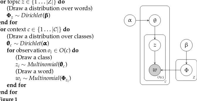
Figure 1 sketches the “generative story” according to which LDA generates arguments for predicates and also presents a plate diagram indicating the dependencies between variables in the model. Table 1 illustrates the semantic representation induced by a 600-topic LDA model trained on predicate–noun co-occurrences extracted from the British National Corpus (for more details of this training data, see Section 4.1). The “semantic classes” are actually distributions over all nouns in the vocabulary rather than a hard partitioning; therefore we present the eight most probable words for each. We also present the contexts most frequently associated with each class. Whereas a

fortopic z∈ {1. . .|Z|}do

(Draw a distribution over words)

Φ

ΦΦz∼Dirichlet(βββ) end for

forcontext c∈ {1. . .|C|}do

(Draw a distribution over classes) θθθc∼Dirichlet(ααα)

forobservation oi∈O(c) do (Draw a class)

zi∼Multinomial(θθθc) (Draw a word) wi∼Multinomial(ΦΦΦzi)

end for end for

α θ

z

w _Φ

β

O(c)

C

Z

Figure 1

Table 1

Sample semantic classes learned by an LDA syntactic co-occurrence model with|Z|=600 trained on BNC co-occurrences.

Class 1

Words:attack, raid, assault, campaign, operation, incident, bombing Object of:launch, carry, follow, suffer, lead, mount, plan, condemn Subject of:happen, come, begin, cause, continue, take, follow Modifies:raid, furnace, shelter, victim, rifle, warning, aircraft

Modified by:heart, bomb, air, terrorist, indecent, latest, further, bombing Prepositional:on home, on house, by force, target for, hospital after, die after

Class 2

Words:line, axis, section, circle, path, track, arrow, curve Object of:draw, follow, cross, dot, break, trace, use, build, cut Subject of:divide, run, represent, follow, indicate, show, join, connect Modifies:manager, number, drawing, management, element, treatment Modified by:straight, railway, long, cell, main, front, production, product Prepositional:on map, by line, for year, line by, point on, in fig, angle to

Class 3

Words:test, examination, check, testing, exam, scan, assessment, sample Object of:pass, carry, use, fail, perform, make, sit, write, apply

Subject of:show, reveal, confirm, prove, consist, come, take, detect, provide Modifies:result, examination, score, case, ban, question, board, paper, kit Modified by:blood, medical, final, routine, breath, fitness, driving, beta Prepositional:subject to, at end, success in, on part, performance on

Class 4

Words:university, college, school, polytechnic, institute, institution, library Object of:enter, attend, leave, visit, become, found, involve, close, grant Subject of:offer, study, make, become, develop, win, establish, undertake Modifies:college, student, library, course, degree, department, school Modified by:university, open, technical, city, education, state, technology Prepositional:student at, course at, study at, lecture at, year at

Class 5

Words:fund, reserve, eyebrow, revenue, awareness, conservation, alarm Object of:raise, set, use, provide, establish, allocate, administer, create Subject of:raise, rise, shoot, lift, help, remain, set, cover, hold

Modifies:manager, asset, raiser, statement, management, commissioner Modified by:nature, pension, international, monetary, national, social, trust Prepositional:for nature, contribution to, for investment, for development

topic model trained on document–word co-occurrences will find topics that reflect broad thematic commonalities, the model trained on syntactic co-occurrences finds semantic classes that capture a much tighter sense of similarity: Words assigned high probability in the same topic tend to refer to entities that have similar properties, that perform similar actions, and have similar actions performed on them. Thus Class 1 is represented by attack, raid, assault, campaign, and so on, forming a coherent semantic grouping. Classes 2, 3, and 4 correspond to groups of tests, geometric objects, and public/educational institutions, respectively. Class 5 has been selected to illustrate a potential pitfall of using syntactic co-occurrences for semantic class induction: fund, revenue, eyebrow, and awareness hardly belong together as a coherent conceptual class. The reason, it seems, is that they are all entities that can be (and in the corpus, are) raised. This class has also conflated different (but related) senses of reserve and as a result the modifier nature is often associated with it.

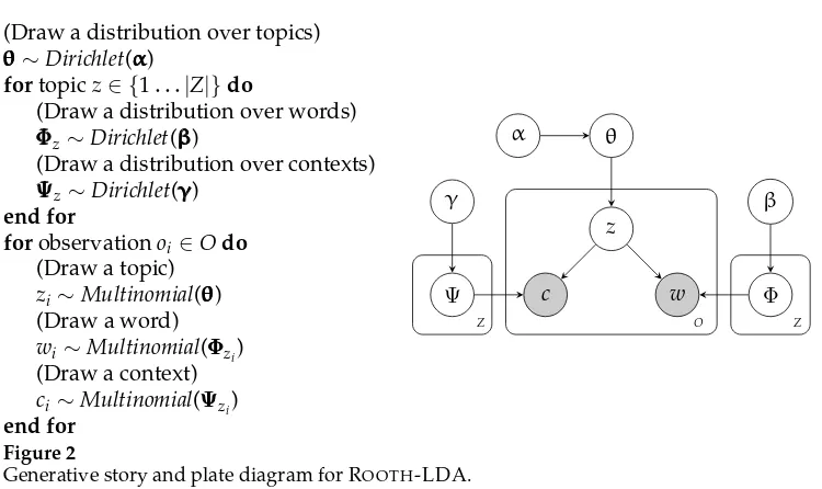
(Draw a distribution over topics) θθθ∼Dirichlet(ααα)

fortopic z∈ {1. . .|Z|}do

(Draw a distribution over words)

Φ

ΦΦz∼Dirichlet(βββ)

(Draw a distribution over contexts)

Ψ

ΨΨz∼Dirichlet(γγγ) end for

forobservation oi∈O do (Draw a topic) zi∼Multinomial(θθθ) (Draw a word) wi∼Multinomial(ΦΦΦzi) (Draw a context) ci∼Multinomial(ΨΨΨzi)

end for

α θ

z

w

c _Φ

β

Ψ γ

O Z

Z

Figure 2

Generative story and plate diagram for ROOTH-LDA.

be “Bayesianized” by placing Dirichlet priors on the component distributions; adapting Equation (25) to our notation, the resulting joint distribution over contexts and words is

P(c, w)=

z

P(c|z)P(w|z)P(z) (27)

The generative story and plate diagram for this model, which was called ROOTH-LDA in ´O S´eaghdha (2010), are given in Figure 2. Whereas LDA induces classes of arguments, ROOTH-LDA induces classes of predicate–argument interactions. Table 2 illustrates some classes learned by ROOTH-LDA from BNC verb–object co-occurrences. One class shows that a cost, number, risk, or expenditure can plausibly be increased, reduced, cut, or involved; another shows that a house, building, home, or station can be built, left, visited, or used. As with LDA, there are some over-generalizations; the fact that an eye or mouth can be opened, closed, or shut does not necessarily entail that it can be locked or unlocked.

For many predicates, the best description of their argument distributions is one that accounts for general semantic regularities and idiosyncratic lexical patterns. This sug-gests the idea of combining a distribution over semantic classes and a predicate-specific

Table 2

Sample semantic classes learned by a Rooth-LDA model with|Z|=100 trained on BNC verb–object co-occurrences.

Class 1 Class 2 Class 3 Class 4

increase cost open door build house spend time

reduce number close eye leave building work day

cut risk shut mouth visit home wait year

involve expenditure lock window use station come hour

control demand slam gate enter church waste night

estimate pressure unlock shop include school take week

limit rate keep fire see plant remember month

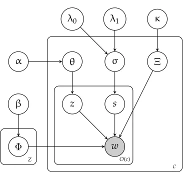
distribution over arguments. One way of doing this is through the model depicted in Figure 3, which we call LEX-LDA; this model defines the selectional preference probability P(w|c) as

P(w|c)=σcPlex(w|c)+(1−σc)Pclass(w|c) (28)

=σcPlex(w|c)+(1−σc)

z

P(w|z)P(z|c) (29)

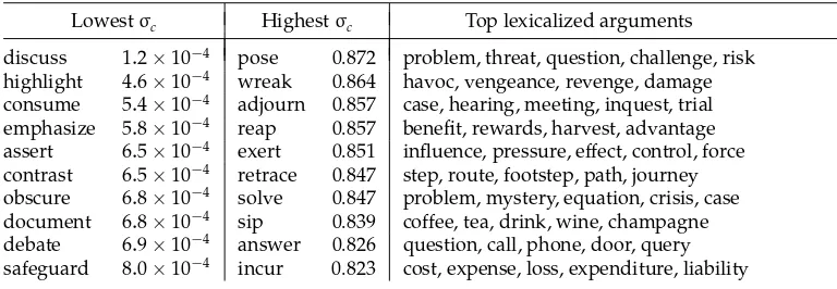
whereσc is a value between 0 and 1 that can be interpreted as a measure of argument lexicalization or as the probability that an observation for context c is drawn from the lexical distribution Plexor the class-based distribution Pclass. Pclasshas the same form as the LDA preference model. The value ofσcwill vary across predicates according to how well their argument preference can be fit by the class-based models; a predicate with highσc will have idiosyncratic argument patterns that are best learned by observing that predicate’s co-occurrences in isolation. In many cases this may reflect idiomatic or non-compositional usages, though it is also to be expected thatσc will correlate with frequency; given sufficient data for a context, smoothing becomes less important. As an example we trained the LEX-LDA model on BNC verb-object co-occurrences and estimated posterior mean values forσcfor all verbs occurring more than 100 times and taking at least 10 different object argument types. The verbs with highest and lowest values are listed in Table 3. Although almost anything can be discussed or highlighted,

fortopic z∈ {1. . .|Z|}do

(Draw a distribution over words)

ΦΦΦz∼Dirichlet(βββ) end for

forcontext c∈ {1. . .|C|}do

(Draw a distribution over topics) θθθc ∼Dirichlet(ααα)

(Draw a distribution over words)

ΞΞΞc ∼Dirichlet(κκκ)

(Draw a lexicalization probability) σc ∼Beta(λ0,λ1)

forobservation oi∈O(c) do

(Draw a lexicalization indicator) si∼Bernoulli(σc)

ifsi=0 then (Draw a topic) zi∼Multinomial(θθθc) (Draw a word) wi∼Multinomial(ΦΦΦzi)

else

(Draw a word) wi∼Multinomial(ΞΞΞc) end if

end for end for

α θ

z s

w β

Φ

σ Ξ

κ λ1

λ0

O(c)

C

Z

Figure 3

Table 3

BNC verbs with lowest and highest estimated lexicalization valuesσcfor their object arguments,

as well as the arguments with highest Plex(w|c) for high-lexicalization verbs.

Lowestσc Highestσc Top lexicalized arguments

discuss 1.2×10−4 _{pose 0.872 problem, threat, question, challenge, risk}

highlight 4.6×10−4 _{wreak 0.864 havoc, vengeance, revenge, damage}

consume 5.4×10−4 _{adjourn 0.857 case, hearing, meeting, inquest, trial}

emphasize 5.8×10−4 _{reap 0.857 benefit, rewards, harvest, advantage}

assert 6.5×10−4 _{exert 0.851 influence, pressure, effect, control, force}

contrast 6.5×10−4 _{retrace 0.847 step, route, footstep, path, journey}

obscure 6.8×10−4 _{solve 0.847 problem, mystery, equation, crisis, case}

document 6.8×10−4 _{sip 0.839 coffee, tea, drink, wine, champagne}

debate 6.9×10−4 _{answer 0.826 question, call, phone, door, query}

safeguard 8.0×10−4 incur 0.823 cost, expense, loss, expenditure, liability

verbs such as pose and wreak have very lexicalized argument preferences. The semantic classes learned by LEX-LDA are broadly comparable to those learned by LDA, though it is less likely to mix classes on the basis of a single argument lexicalization; whereas the LDA class in row 5 of Table 1 is distracted by the high-frequency collocations nature reserve and raise eyebrow, LEX-LDA models trained on the same data can explain these through lexicalization effects and separate out body parts, conservation areas, and investments in different classes.

3.4 Parameter and Hyperparameter Learning

3.4.1 Learning Methods. A variety of methods are available for parameter learning in Bayesian models. The two standard approaches are variational inference, in which an approximation to the true distribution over parameters is estimated exactly, and sampling, in which convergence to the true posterior is guaranteed in theory but rarely verifiable in practice. In some cases the choice of approach is guided by the model, but often it is a matter of personal preference; for LDA, there is evidence that equivalent levels of performance can be achieved through variational learning and sampling given appropriate parameterization (Asuncion et al. 2009). In this article we use learning methods based on Gibbs sampling, following Griffiths and Steyvers (2004). The basic idea of Gibbs sampling is to iterate through the corpus one observation at a time, updating the latent variable value for each observation according to the conditional probability distribution determined by the current observed and latent variable values for all other observations. Because the likelihoods are multinomials with Dirichlet priors, we can integrate out their parameters using Equation (21).

For LDA, the conditional probability that the latent variable for the ith observation is assigned value z is computed as

P(zi=z|z−i, ci, wi)∝( fzci+αz)

fzwi+β fz+|W|β

(30)

For ROOTH-LDA we make a similar calculation:

P(zi=z|z−i, ci, wi)∝( fz+αz)

fzwi +β fz+|W|β

fzci+β

fz+|C|γ (31)

For LEX-LDA the lexicalization variables simust also be sampled for each token. We “block” the sampling for zi and si to improve convergence. The Gibbs sampling distribution is

P(si=0, zi=z|z−i, s−i, ci, wi)∝( fci,s=0+λ0)

fzci+αz fci,s=0+

zαz

fzwi+β

fz+|W|β (32)

P(si=1, zi=∅|z−i, s−i, ci, wi)∝( fci,s=1+λ1)

fciwi,s=1+κ fci,s=1+|W|κ

(33)

P(si=0, zi=∅|z−i, s−i, ci, wi)=0 (34)

P(si=1, zi=∅|z−i, s−i, ci, wi)=0 (35)

where∅indicates that no topic is assigned. The fact that topics are not assigned for all tokens means that LEX-LDA is less useful in situations that require representational power they afford—for example, the contextual similarity paradigm described in Section 3.5.

A naive implementation of the sampler will take time linear in the number of topics and the number of observations to complete one iteration. Yao, Mimno, and McCallum (2009) present a new sampling algorithm for LDA that yields a considerable speedup by reformulating Equation (30) to allow caching of intermediate values and an intelligent sorting of topics so that in many cases only a small number of topics need be iterated though before assigning a topic to an observation. In this article we use Yao, Mimno, & McCallum’s algorithm for LDA, as well as a transformation of the ROOTH-LDA and LEX-LDA samplers that can be derived in an analogous fashion.

3.4.2 Inference. As noted previously, the Gibbs sampling procedure is guaranteed to converge to the true posterior after a finite number of iterations; however, this number is unknown and it is difficult to detect convergence. In practice, we run the sampler for a hopefully sufficient number of iterations and perform inference based on the final sampling state (assignments of all z and s variables) and/or a set of intermediate sampling states.

In the case of the LDA model, the selectional preference probability P(w|c) is estimated using posterior mean estimates ofθcandΦz:

P(w|c)=

z

P(z|c)P(w|z) (36)

P(z|c)= fzc+αz fc+

zαz

(37)

P(w|z)= fzw+β

For ROOTH-LDA, the joint probability P(c, w) is given by

P(c, w)=

z

P(c|z)P(w|z)P(z) (39)

P(z)= fz+αz

|O|+_zαz (40)

P(w|z)= fzw+β fz+|W|β

(41)

P(c|z)= fzc+γ

fz+|C|γ (42)

For LEX-LDA, P(w|c) is given by

P(w|c)=P(σ=1|c)Plex(w|c)+P(σ=0|c)Pclass(w|c) (43)

P(σ=1|c)= fc,s=1+λ1

fc+λ0+λ1 (44)

P(σ=0|c)=1−P(σ=1|c) (45)

Plex(w|c)=

fwc,s=1+κ

fc,s=1+|W|κ (46)

Pclass(w|c)=

z

P(z|c)P(w|z) (47)

P(z|c)= fzc+αz fc,s=0+

zαz

(48)

P(w|z)= fzw+β

fz+|W|β (49)

Given a sequence or chain of sampling states S1,. . ., Sn, we can predict a value for

P(w|c) or P(c, w) using these equations and the set of latent variable assignments at a single state Si. As the sampler is initialized randomly and will take time to find a good area of the search space, it is standard to wait until a number of iterations have passed before using any samples for prediction. States S1,. . ., Sb from this burn-in period are discarded.

For predictive stability it can be beneficial to average over predictions computed from more than one sampling state; for example, we can produce an averaged estimate of P(w|c) from a set of states S:

P(w|c)= 1

|S|

Si∈S

PSi(w|c) (50)

3.4.3 Choosing |Z|. In the “parametric” latent variable models used here the number of topics or semantic classes, |Z|, must be fixed in advance. This brings significant efficiency advantages but also the problem of choosing an appropriate value for|Z|. The more classes a model has, the greater its capacity to capture fine distinctions between entities. However, this finer granularity inevitably comes at a cost of reduced general-ization. One approach is to choose a value that works well on training or development data before evaluating held-out test items. Results in lexical semantics are often reported over the entirety of a data set, meaning that if we wish to compare those results we cannot hold out any portion. If the method is relatively insensitive to the parameter it may be sufficient to choose a default value. Rooth et al. (1999) suggest cross-validating on the training data likelihood (and not on the ultimate evaluation measure). An alter-native solution is to average the predictions of models trained with different choices of|Z|; this avoids the need to pick a default and can give better results than any one value as it integrates contributions at different levels of granularity. As mentioned in Section 3.4.2 we must take care when averaging predictions to compute with quan-tities that do not rely on topic identity—for example, estimates of P(a|p) can safely be combined whereas estimates of P(z1|p) cannot.

3.4.4 Hyperparameter Estimation. Although the likelihood parameters can be integrated out, the parameters for the Dirichlet and Beta priors (often referred to as “hyperparame-ters”) cannot and must be specified either manually or automatically. The value of these parameters affects the sparsity of the learned posterior distributions. Furthermore, the use of an asymmetric prior (where not all its parameters have equal value) implements an assumption that some observation values are more likely than others before any observations have been made. Wallach, Mimno, and McCallum (2009) demonstrate that the parameterization of the Dirichlet priors in an LDA model has a material effect on performance, recommending in conclusion a symmetric prior on the “emission” likelihood P(w|z) and an asymmetric prior on the document topic likelihoods P(z|d). In this article we follow these recommendations and, like Wallach, Mimno, and McCallum, we optimize the relevant hyperparameters using a fixed point iteration to maximize the log evidence (Minka 2003; Wallach 2008).

3.5 Measuring Similarity in Context with Latent-Variable Models

The representation induced by latent variable selectional preference models also allows us to capture the disambiguatory effect of context. Given an observation of a word in a context, we can infer the most probable semantic classes to appear in that context and we can also infer the probability that a class generated the observed word. We can also estimate the probability that the semantic classes suggested by the observation would have licensed an alternative word. Taken together, these can be used to estimate in-context semantic similarity. The fundamental intuitions are similar to those behind the vector-space models in Section 2.3.2, but once again we are viewing them from the perspective of probabilistic modeling.

The basic idea is that we identify the similarity between an observed term woand an alternative term wsin context C with the similarity between the probability distribution over latent variables associated with wo and C and the probability distribution over latent variables associated with ws:

This assumes that we can associate a distribution over the same set of latent variables with each context item c∈C. As noted in Section 2.3.2, previous research has found that conditioning the representation of both the observed term and the candidate substitute on the context gives worse performance than conditioning the observed term alone; we also found a similar effect. Dinu and Lapata (2010) present a specific version of this framework, using a window-based definition of context and the assumption that the similarity given a set of contexts is the product of the similarity value for each context:

simDL10(wo, ws|C)=

c∈C

sim(P(z|wo, c), P(z|ws)) (52)

In this article we generalize to syntactic as well as window-based contexts and also derive a well-motivated approach to incorporating multiple contexts inside the prob-ability model; in Section 4.5 we show that both innovations contribute to improved performance on a lexical substitution data set.

The distributions we use for prediction are as follows. Given an LDA latent variable preference model that generates words given a context, it is straightforward to calculate the distribution over latent variables conditioned on an observed context–word pair:

PC→T(z|wo, c)= P(wo|z)P(z|c)

zP(wo|z)P(z|c) (53)

Given a set of multiple contexts C, each of which has an opinion about the distribution over latent variables, this becomes

P(z|wo, C)=

P(wo|z)P(z|C)

zP(wo|z)P(z|C)

(54)

P(z|C)=

c∈CP(z|c)

z

c∈CP(z|c)

(55)

The uncontextualized distribution P(z|ws) is not given directly by the LDA model. It can be estimated from relative frequencies in the Gibbs sampling state; we use an unsmoothed estimate.8 _{We denote this model C→T to note that the target word is} generated given the context.

Where the context–word relationship is asymmetric (as in the case of syntactic dependency contexts), we can alternatively learn a model that generates contexts given a target word; we denote this model T→C:

PT→C(z|wo, c)=

P(z|wo)P(c|z)

zP(z|wo)P(c|z)

(56)

Again, we can generalize to non-singleton context sets:

P(z|wo, C)= P(z|wo)P(C|z)

zP(z|wo)P(C|z) (57)

where

P(C|z)=

c∈C

P(c|z) (58)

Equation (57) has the form of a “product of experts” model (Hinton 2002), though unlike many applications of such models we train the experts independently and thus avoid additional complexity in the learning process. The uncontextualized distribution P(z|ws) is an explicit component of the T→C model.

An analogous definition of similarity can be derived for the ROOTH-LDA model. Here there is no asymmetry as the context and target are generated jointly. The distri-bution over topics for a context c and target word wois given by

PROOTH-LDA(z|wo, c)=

P(wo, c|z)P(z)

zP(wo, c|z)P(z) (59)

while calculating the uncontextualized distribution P(z|ws) requires summing over the set of possible contexts C’:

PROOTH-LDA(z|ws)=

P(z)_c∈CP(ws, c|z)

zP(z)

c∈CP(ws, c|z) (60) Because the interaction classes learned by ROOTH-LDA are specific to a relation type, this model is less applicable than LDA to problems that involve a rich context set C.

Finally, we must choose a measure of similarity between probability distributions. The information theory literature has provided many such measures; in this article we use the Bhattacharyya coefficient (Bhattacharyya 1943):

simbhatt(Px(z), Py(z))=

z

Px(z)Py(z) (61)

One could alternatively use similarities derived from probabilistic divergences such as the Jensen–Shannon Divergence or the L1 distance (Lee 1999; ´O S´eaghdha and Copestake 2008).

3.6 Related Work

words; however, their model does not encourage sharing of classes between different predicates. Reisinger and Mooney (2011) propose a very interesting variant of the latent-variable approach in which different kinds of contextual behavior can be explained by different “views,” each of which has its own distribution over latent variables; this model can give more interpretable classes than LDA for higher settings of|Z|.

Some extensions of the LDA topic model incorporate local as well as document context to explain lexical choice. Griffiths et al. (2004) combine LDA and a hidden Markov model (HMM) in a single model structure, allowing each word to be drawn from either the document’s topic distribution or a latent HMM state conditioned on the preceding word’s state; Moon, Erk, and Baldridge (2010) show that combining HMM and LDA components can improve unsupervised part-of-speech induction. Wallach (2006) also seeks to capture the influence of the preceding word, while at the same time generating every word from inside the LDA model; this is achieved by conditioning the distribution over words on the preceding word type as well as on the chosen topic. Boyd-Graber and Blei (2008) propose a “syntactic topic model” that makes topic selection conditional on both the document’s topic distribution and on the topic of the word’s parent in a dependency tree. Although these models do represent a form of local context, they either use a very restrictive one-word window or a notion of syntax that ignores lexical or dependency-label effects; for example, knowing that the head of a noun is a verb is far less informative than knowing that the noun is the direct object of eat.

More generally, there is a connection between the models developed here and latent-variable models used for parsing (e.g., Petrov et al. 2006). In such models each latent state corresponds to a “splitting” of a part-of-speech label so as to pro-duce a finer-grained grammar and tease out intricacies of word–rule “co-occurrence.” Finkel, Grenager, and Manning (2007) and Liang et al. (2007) propose a non-parametric Bayesian treatment of state splitting. This is very similar to the motivation behind an LDA-style selectional preference model. One difference is that the parsing model must explain the parse tree structure as well as the choice of lexical items; another is that in the selectional preference models described here each head–dependent relation is treated as an independent observation (though this could be changed). These differences allow our selectional preference models to be trained efficiently on large corpora and, by fo-cusing on lexical choice rather than syntax, to home in on purely semantic information. Titov and Klementiev (2011) extend the idea of latent-variable distributional modeling to do “unsupervised semantic parsing” and reason about classes of semantically similar lexicalized syntactic fragments.

4. Experiments 4.1 Training Corpora

In our experiments we use two training corpora:

BNC the written component of the British National Corpus,9 comprising around 90 million words. The corpus was tagged for part of speech, lemmatized, and parsed with the RASP toolkit (Briscoe, Carroll, and Watson 2006).

COORDINATION:

Cats and

c:conj:n

OO

c:conj:n

OO

dogs run v:ncsubj:n

⇒ Cats and dogs_OO

n:and:n

OO run v:ncsubj:n

PREDICATION:

The cat is

v:ncsubj:n

OO

v:xcomp:j

fierce _⇒ The cat

n:ncmod:j

is fierce

PREPOSITIONS:

The cat n:ncmod:i

in

i:dobj:n

OO

the hat ⇒ The cat

n:prep in:n

in the hat

Figure 4

Dependency graph preprocessing.

WIKI a Wikipedia dump of over 45 million sentences (almost 1 billion words) tagged, lemmatized, and parsed with the C+C toolkit10_{and the fast CCG parser described} by Clark et al. (2009).

Although two different parsers were used, they both have the ability to output gram-matical relations in the RASP format and hence they are interoperable for our purposes as downstream users. This allows us to construct a combined corpus by simply concate-nating the BNC and WIKI corpora.

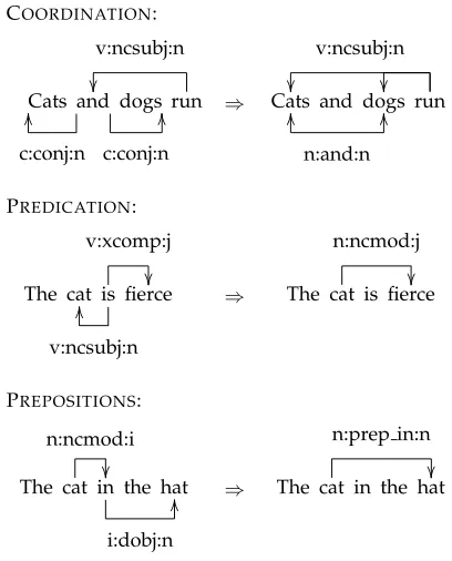
In order to train our selectional preference models, we extracted word–context observations from the parsed corpora. Prior to extraction, the dependency graph for each sentence was transformed using the preprocessing steps illustrated in Figure 4. We then filtered for semantically discriminative information by ignoring all words with part of speech other than common noun, verb, adjective, and adverb. We also ignored instances of the verbs be and have and discarded all words containing non-alphabetic characters and all words with fewer than three characters.11

As mentioned in Section 2.1, the distributional semantics framework admits flex-ibility in how the practitioner defines the context of a word w. We investigate two possibilities in this article:

Syn The context of w is determined by the syntactic relations r and words wincident to it in the sentence’s parse tree, as illustrated in Section 3.1.

10http://svn.ask.it.usyd.edu.au/trac/candc.

Win5 The context of w is determined by the words appearing within a window of five words on either side of it. There are no relation labels, so there is essentially just one relation r to consider.

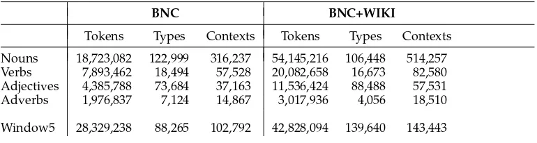
Training topic models on a data set with very large “documents” leads to tractability issues. The window-based approach is particularly susceptible to an explosion in the number of extracted contexts, as each token in the data can contribute 2×W word– context observations, where W is the window size. We reduced the data by applying a simple downsampling technique to the training corpora. For the WIKI/Syn corpus, all word–context counts were divided by 5 and rounded to the nearest integer. For the WIKI/Win5 corpus we divided all counts by 70; this number was suggested by Dinu and Lapata (2010), who used the same ratio for downsampling the similarly sized English Gigaword Corpus. Being an order of magnitude smaller, the BNC required less pruning; we divided all counts in the BNC/Win5 by 5 and left the BNC/Syn corpus unaltered. Type/token statistics for the resulting sets of observations are given in Table 4.

4.2 Evaluating Selectional Preference Models

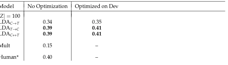
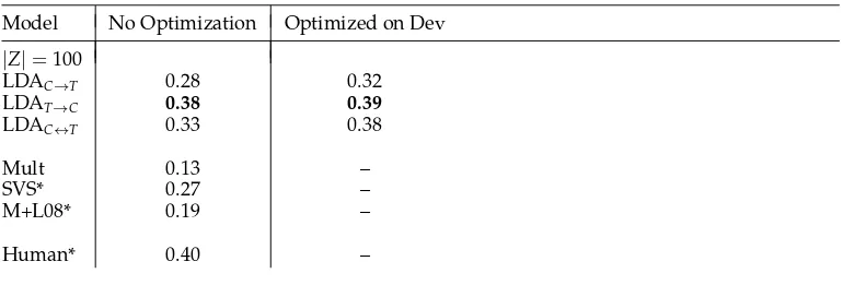
Various approaches have been suggested in the literature for evaluating selectional preference models. One popular method is “pseudo-disambiguation,” in which a sys-tem must distinguish between actually occurring and randomly generated predicate– argument combinations (Pereira, Tishby, and Lee 1993; Chambers and Jurafsky 2010). In a similar vein, probabilistic topic models are often evaluated by measuring the probability they assign to held-out data; held-out likelihood has also been used for evaluation in a task involving selectional preferences (Schulte im Walde et al. 2008). These two approaches take a “language modeling” approach in which model quality is identified with the ability to predict the distribution of co-occurrences in unseen text. Although this metric should certainly correlate with the semantic quality of the model, it may also be affected by frequency and other idiosyncratic aspects of language use unless tightly controlled. In the context of document topic modeling, Chang et al. (2009) find that a model can have better predictive performance on held-out data while inducing topics that human subjects judge to be less semantically coherent.

In this article we choose to evaluate models by comparing system predictions with semantic judgments elicited from human subjects. These judgments take various forms. In Section 4.3 we use judgments of how plausible it is that a given predicate takes a given word as its argument. In Section 4.4 we use judgments of similarity

Table 4

Type and token counts for the BNC and BNC+WIKI corpora.

BNC BNC+WIKI

Tokens Types Contexts Tokens Types Contexts

Nouns 18,723,082 122,999 316,237 54,145,216 106,448 514,257

Verbs 7,893,462 18,494 57,528 20,082,658 16,673 82,580

Adjectives 4,385,788 73,684 37,163 11,536,424 88,488 57,531

Adverbs 1,976,837 7,124 14,867 3,017,936 4,056 18,510