A Flexible, Corpus Driven Model of Regular and Inverse Selectional Preferences

and Inverse Selectional Preferences

Katrin Erk

University of Texas at Austin

Sebastian Padó

Ulrike Padó

Vico Research and Consulting GmbH

We present a vector space–based model for selectional preferences that predicts plausibility scores for argument headwords. It does not require any lexical resources (such as WordNet). It can be trained either on one corpus with syntactic annotation, or on a combination of a small semantically annotated primary corpus and a large, syntactically analyzed generalization cor-pus. Our model is able to predict inverse selectional preferences, that is, plausibility scores for predicates given argument heads.

We evaluate our model on one NLP task (pseudo-disambiguation) and one cognitive task (prediction of human plausibility judgments), gauging the influence of different parameters and comparing our model against other model classes. We obtain consistent benefits from using the disambiguation and semantic role information provided by a semantically tagged primary cor-pus. As for parameters, we identify settings that yield good performance across a range of experi-mental conditions. However, frequency remains a major influence of prediction quality, and we also identify more robust parameter settings suitable for applications with many infrequent items.

1. Introduction

Selectional preferencesorselectional constraintsdescribe knowledge about possible and plausible fillers for a predicate’s argument positions. They model the fact that there is often a semantically coherent set of concepts that can fill a given argument posi-tion. Selectional preferences can help for many text analysis tasks which involve com-paring different attachment decisions. Examples include syntactic disambiguation (Hindle and Rooth 1993; Toutanova et al. 2005), word sense disambiguation (WSD,

∗Department of Linguistics, Calhoun Hall 512, 1 University Station B 5100, Austin, TX 78712. E-mail:[email protected].

∗∗E-mail:[email protected]. †E-mail:[email protected].

McCarthy and Carroll 2003), semantic role labeling (SRL, Gildea and Jurafsky 2002), and characterizing the conditions under which entailment holds between two predicates (Zanzotto, Pennacchiotti, and Pazienza 2006; Pantel et al. 2007). Furthermore, selec-tional preferences are also helpful for determining linguistic properties of predicates and predicate–argument combinations, for example in compositionality assessment (McCarthy, Venkatapathy, and Joshi 2007) or the detection of diathesis alternations (McCarthy 2000). In psycholinguistics, selectional preferences predict human plausibil-ity judgments for predicate–argument combinations (Resnik 1996) and effects in human sentence reading times (Padó, Crocker, and Keller 2009).

All these applications rely on the availability of broad-coverage, reliable selectional preferences for predicates and their argument positions. Given the immense effort nec-essary for manual semantic lexicon building and its associated reliability problems (see, e.g., Briscoe and Boguraev 1989), all contemporary models of selectional preferences acquire selectional preferences automatically from large corpora.

The simplest strategy is to extract triples (v,r,a) of a predicate, role, and argument headword (or filler) from a corpus, and then to compute selectional preference as relative frequencies. However, due to the Zipfian nature of word frequencies, the first step on its own results in a very sparse list of headwords, in particular for less frequent predicates. As an example, the verbanglicize only appears with nine direct objects in the 100-million word British National Corpus (BNC, Burnard 1995). Only one of them, name, appears more than once. Many highly plausible fillers are missing from the list, such aswordorspelling.

In order to make sensible predictions for triples that are unseen at training time, it is crucial to add a generalization step that infers a degree of preference for new, unseen headwords for a given predicate and role.1 _{The result is, in the ideal case, an} assignment to every possible headword of some degree of compatibility (or plausibil-ity) with the predicate’s preferences. In the case ofanglicize, the desired result would be a high plausibility for words like the (previously seen)wordlistandsurnameas well as the (unseen)wordandspelling, and a low plausibility for (likewise unseen) words like cowandmachine.

The predominant approach to generalizing over headwords, first introduced by Resnik (1996), is based on semantic hierarchies such as WordNet (Miller et al. 1990). The idea is to map all observed headwords onto synsets, and then generalize to a characteri-zation of the selectional preference in terms of the WordNet noun hierarchy. This can be achieved in many different ways (Abe and Li 1996; Resnik 1996; Ciaramita and Johnson 2000; Clark and Weir 2001). The performance of these models relies on the coverage of the lexical resources, which can be a problem even for English (Gildea and Jurafsky 2002). An alternative approach to generalization usesco-occurrence information, either in the form of distributional models or through a clustering approach. These models, which avoid dependence on lexical resources, use corpus data for generalization (Dagan, Lee, and Pereira 1999; Rooth et al. 1999; Bergsma, Lin, and Goebel 2008).

In this article, we present a lightweight model for the acquisition and representa-tion of selecrepresenta-tional preferences. Our model is fully distriburepresenta-tional and does not require any knowledge sources beyond a large corpus where subjects and objects can be iden-tified with reasonable accuracy. Its key point is to use vector space similarity (Lund and Burgess 1996; Laundauer and Dumais 1997) to generalize from seen to unseen

headwords. The vector space representations which serve as a basis for computing similarity can in principle be computed from any arbitrary corpus, given that it is large enough. In particular, this need not be the same corpus as the one on which we observe predicate–headword co-occurrences. Our model thus distinguishes between aprimary corpus, from which the predicate–role–headword triples are extracted, and a generali-zation corpusfor computing the vector space representations. This distinction makes it possible to apply our model to primary corpora with rich information that are too small for efficient generalization, such as domain-specific corpora or corpora with deeper linguistic analysis, as long as a larger, even if potentially noisier, generalization corpus is available. We empirically demonstrate the benefit of this distinction. We use FrameNet (Fillmore, Johnson, and Petruck 2003) as primary corpus and the BNC as generalization corpus, modeling selectional preferences for semantic roles with near-perfect coverage and low error rate.2

We evaluate our model on two tasks. The first task is pseudo-disambiguation (Yarowsky 1993), where the model decides which of two randomly chosen words is a better filler for the given argument position. This task tests model properties that are needed for concrete semantic analysis tasks, most notably word sense disambiguation, but also for semantic role labeling. The second task is the prediction of human plausibility ratings, which is a standard task-independent benchmark for the quality of selectional preferences. We test our model across a range of parameter settings to identify best-practice values and show that it robustly outperforms both WordNet-based and other distributional models on both tasks.

Finally, we investigate inverse preferences, that is, preferences that arguments have for their predicates. Although there is ample cognitive evidence for the existence of such preferences (e.g., McRae et al. 2005), to our knowledge, they have not been in-vestigated systematically in linguistics. However, statistics about inverse preferences have been used implicitly in computational linguistics (e.g., Hindle 1990; Rooth et al. 1999). We investigate the properties of inverse selectional preferences in comparison to regular selectional preferences, and show that it is possible to predict inverse prefer-ences with our selectional preference model as well.

The model that we discuss in this article, EPP, was first introduced in Erk (2007) (using a pseudo-disambiguation task for evaluation) and further studied by Padó, Padó, and Erk (2007) (evaluating against human plausibility judgments). In the current text, we perform a more extensive evaluation and analysis, including the new evaluation on inverse preferences, and we introduce a new similarity measure, nGCM, which achieves excellent performance in many settings.

2. Computational Models of Selectional Preferences

In this section, we provide an overview of corpus-based models of selectional prefer-ences. See Table 1 for a summary of the notation that we use.

Table 1

Notation used throughout the article.

w∈Lemmas Word. We assume lemmatization throughout.

v∈Preds Predicate.Predsmay be a subset ofLemmas, or a set of semantic classes.

r∈Roles Role/Argument slot.Rolesmay be a set of grammatical functions, or of semantic roles.

a∈Args⊆Lemmas (Potential) argumentheadword.

c∈C Semantic class on which selectional preferences are

conditioned, for example, WordNet sense, FrameNet frame, or latent semantic class.

VS=(DTrans,

Basis,sim,STrans)

Vector space.Basisis a set of basis elements,sima similarity measure,DTransa transformation of raw counts, andSTrans

a transformation of the space.

We write w=wb1,. . .,wbn for the representation of w∈ Lemmasin a vector space withBasis={b1,. . .,bn}.

wtr,v(a) Weightof argument headwordafor predicatevand roler.

2.1 Historical Models

In formal linguistics, selectional restrictions were employed as strict Boolean restrictions by Katz and Postal (Katz and Fodor 1963; Katz and Postal 1964) as input to a mutual dis-ambiguation process between predicates and their modifiers. Sentences are semantically anomalous if there are no mutually consistent readings for the two words. Semantically anomalous sentences would receive no reading, whereas ambiguous sentences would receive several readings.

The strict dismissal as meaningless of sentences that violate selectional restrictions was later criticized. A case in point is metaphors, which often combine predicates and arguments from different domains (Lakoff and Johnson 1980). Wilks (1975:329) stated that “rejecting utterances is just what humans do not. They try to understand them.” He proposes to reconceptualize selectional restrictions as preferences whose violation is dispreferred, but not fatal. His proposal for a semantic interpretation mechanism still uses semantic primitives, but always produces a single most plausible interpretation by choosing the senses of each word that maximize the compatibility between selectional preferences and semantic types. In this manner, he is able to compute semantic repre-sentations for sentences that violate selectional restrictions, including metaphors such as “my car drinks gasoline.”

2.2 Semantic Hierarchy–Based Models

The first broad-coverage computational model of selectional preferences, and still one of the best-known ones, namely that of Resnik (1996), belongs to the class of semantic hierarchy–based models. These models generalize over observed headwords using a semantic hierarchy or ontology for nouns. The two main advantages of such models are that (a) they can make predictions for all words covered by the hierarchy, even for very infrequent ones for which distributional representations tend to be unreliable; and (b) the hierarchy robustly guides generalization even for few observed headwords.

concen-trates on selectional preferences for subjects and objects. For the generalization step, Resnik’s model maps all headwords onto WordNet synsets (or classes) c. Resnik first computes the overallselectional preference strengthfor each verb–relation pair (v,r), that is, the degree to which the pair constrains possible fillers. To estimate this quantity, the distribution of WordNet synsets for this particular verb–relation pair is compared to the distribution of synsets over all verbs, given the relation r. Technically, this is achieved using Kullback–Leibler divergence:

SelStr(v,r)=D(P(c|v,r)||P(c|r))=

c∈C

P(c|v,r)log(P(c|v,r)

P(c|r) ) (1)

The parametersP(c|v,r) andP(c|r) are estimated from the corpus frequencies of tuples (v,r,a) and the membership of nounsain WordNet classesc: The observed frequency of (v,r,a) is split equally among all WordNet classes for a. This avoids word sense disambiguration, but incurs a certain share of wrong attributions. The intuition of SelStr(v,r) is that a verb–relation pair that only allows a limited range of argument heads will have a posterior distribution over classes that strongly diverges from the prior.

Next, theselectional associationof the triple,SelAssoc(v,r,c), is computed as the ratio of the selectional preference strength for this particular classcto the overall selec-tional preference strength of the verb–relation pair (v,r). This is shown in Equation (2).

SelAssoc(v,r,c)= P(c|v,r)log

P(c|v,r) P(c|r)

SelStr(v,r) (2)

Finally, the selectional preference between a verb, a relation, and an argument head is defined as the maximal selectional association of the verb, the relation, and any WordNet class c that the argument can instantiate. We will refer to this model as

RESNIKherein.

In subsequent years, a number of WordNet-based models were developed that differ from Resnik’s model in the details of how the generalization in the WordNet hierarchy is performed. Abe and Li (1996) characterize selectional preferences by a tree cut through the WordNet noun hierarchy that minimizes tree cut length while maximizing accuracy of prediction. Clark and Weir (2001) perform generalization by ascending the WordNet noun hierarchy as long as the degree of selectional preference among siblings is not significantly different. Ciaramita and Johnson (2000) encode WordNet in a Bayesian Network to take advantage of the Bayes nets’ ability to “ex-plain away” ambiguity. Grishman and Sterling (1992) perform generalization on the basis of a manually constructed semantic hierarchy specifically developed on the same corpus.

2.3 Distributional Models

semantic hierarchy–based models, usually use grammatical functions as the setRoles

for which selectional preferences are predicted.

Pereira, Tishby, and Lee (1993) and Rooth et al. (1999) generalize by discovering latent classes of noun–verb pairs with soft clustering. They model the probability of a word a as the argument of a predicate v as the probability of generating v and a independently from the latent classesc:

P(v,a)=

c∈C

P(c,v,a)=

c∈C

P(c)P(v|c)P(a|c) (3)

Pereira, Tishby, and Lee (1993) develop a task-specific procedure to optimize P(c), P(v|c), andP(a|c). Their procedure supports hierarchical clustering and can optimize the number of clusters. Rooth et al. (1999) present a simpler Expectation Maximization– based estimation procedure which takes the number of clusters as input parameter. We refer to this model asROOTH ET AL.herein.

Dagan, Lee, and Pereira (1999) introduce a general model for computing co-occurrence probabilities with similarity-based smoothing. Although not intended as a model of selectional preferences, it can also be interpreted as such. Given a similarity measuresimdefined on word pairs, they compute the smoothed occurrence probability of a wordw2givenw1as

Psim(w2|w1)=

w∈Simset(w1)

sim(w1,w)

Z(w1) P(w2|w) (4)

where Simset(w) is the set of words most similar towaccording to sim, and Z(w1)=

w∈Simset(w1)sim(w1,w) is a normalizing factor. This model predicts w2 given w1 by backing off fromw1to wordswsimilar tow1. The contribution of eachwin predicting P(w2|w1) is weighted by sim(w1,w). The similarity sim(w1,w) is computed on vector space representations.

Recently, Bergsma, Lin, and Goebel (2008) have adopted a discriminative ap-proach to the prediction of selectional preferences. The features they use are mainly co-occurrence statistics, enriched with morphological context features to alleviate sparse data problems for low-frequency argument heads. They train one SVM per verb– argument position pair, using unobserved verb–argument combinations as negative examples, which makes their approach independent of manually annotated training data. Schulte im Walde et al. (2008) present a model that combines features of the semantic hierarchy–based and the distributional approaches by integrating WordNet into an EM-based clustering model; Schulte im Walde (2010) shows that integrating noun–modifier relations improves the prediction of human plausibility judgments.

2.4 Semantic Role–Based Models

would. These advantages, however, come at the cost of considerably greater sparsity issues.

Padó, Crocker, and Keller (2009) present a model based on FrameNet (Fillmore, Johnson, and Petruck 2003). This model estimates selectional preferences with a gen-erative probability model that equates the plausibility of a (v,r,a) triple with the joint probability of observing the thematic roler, the verbv, and the argumenta, plus the verb’s FrameNet sense cand the grammatical functiongf of the argument. This joint probability can be decomposed using the chain rule:

P(v,c,r,gf,a)=P(v)P(c|v)P(r|v,c)P(gf|r,v,c)P(a|gf,r,v,c) (5)

The model does not make any independence assumptions. To counteract sparse data issues for the more complex terms, the model applies WordNet-based generalization (for nouns), distributional clustering (for verbs), and Good–Turing smoothing. We refer to this model as PADO ET AL.Another semantic role–based model was proposed by Vandekerckhove, Sandra, and Daelemans (2009). It acquires selectional preferences for PropBank roles from a PropBank-labeled corpus, generalizing to unseen headwords with memory-based learning.

3. A Distributional Exemplar-Based Model of Selectional Preferences:EPP

We now present the EPP model of selectional preferences. It falls into the category of distributional models. More specifically, it is an exemplar model that remembers all seen headwords for a given argument position and computes the degree of plausibility for a new headword candidate through its similarity to the stored exemplars. Exemplars are modeled as vectors in a semantic space.

Exemplar models are a well-known modeling framework that is used in psychol-ogy (Nosofsky 1986), in computational linguistics (under the name of memory-based learning [Daelemans and van der Bosch 2005]), and in linguistics, particularly phonet-ics (Hay, Nolan, and Drager 2006). The appeal of exemplar models is that they provide a cognitively plausible process of learning as storing exemplars, and categorization as similarity computation that is grounded in features of the exemplars (e.g., formants in phonetics, and contexts in lexical semantics).

The representation of selectional preferences through feature vectors also fits in well with work in psycholinguistics by McRae, Ferretti, and Amyote (1997), who studied the characterization of verb selectional preferences through features elicited from human subjects. They found high overlap between features used to characterize the selectional preferences on the one hand, and features listed for typical role fillers on the other hand. For example, features generated for the agent role offrightenincludemean,scary, and ugly, features that were also highly relevant for the typical filler nounmonster.

3.1 The Model

As stated previously, we assume that we have two corpora which assume different func-tions in the model: the primary corpus, which provides information about predicate– argument co-occurrences but may be too sparse for generalization; and the large, but potentially noisy, generalization corpus, from which we obtain reliable semantic simi-larity estimates.

Thus, the first step is the extraction of triples (v,r,a) of a predicate v∈Preds, a relationr∈Roles, and a headworda∈Argsfrom the primary corpus. LetSeenargs(r,v) be the set of argument headwords seen with an argument position rof a predicate v in the primary corpus. Given these triples, we predict the plausibility for an arbitrary noun a0 in position (v,r) through the semantic similarity of a0 to all the members of Seenargs(r,v). We obtain these similarity ratings by first computing vector space representations for both and the members ofseen(r,v) from the generalization corpus, and then using a standard vector space similarity measure. We compute the plausibility fora0as

SelprefEPP_r,v(a0)=

a∈Seenargs(r,v) wtr,v(a)

Zr,v ·sim(a0,a) (6)

where sim(a0,a) is the similarity between the vector space representations of a0 and a,wtr,v(a) a weight for the seen headworda, andZr,v a normalization constant, Zr,v=

a∈Seenargs(r,v)wtr,v(a), so that the number of observed exemplars for each (v,r) pair does not matter. BecauseSelprefEPPis basically a weighted average over similarity values, the range ofSelprefEPPis identical to the range of the employed similarity functionsim. For example, the range is [−1, 1] for cosine similarity, or [0, 1] for the Jaccard coefficient (cf. Section 3.3). We discuss possible choices of both the similaritysimand the weightwtr,v in Section 3.3.

3.2 Vector Space Representations

We use vector space representations for generalization. In a vector space model, each target wordis represented as a vector, typically constructed from co-occurrence counts with context words in a large corpus (the so-calledbasis elements). The underlying assumption, which goes back to Firth (1957) and Harris (1968), is that words with similar meanings occur in similar contexts and will be assigned similar vectors. Thus, the distance between the vectors of two target words, as given by some distance measure (e.g., Cosine or Jaccard), reflects theirsemantic similarity.

Vector space models are simple to construct, and the semantic similarity they pro-vide has found a wide range of applications. Examples in NLP include information retrieval (Salton, Wong, and Yang 1975), automatic thesaurus extraction (Grefenstette 1994), and predominant sense identification (McCarthy et al. 2004). Lexical resources based on distributional similarity (e.g., Lin [1998]’s thesaurus) are used in a wide range of applications that profit from knowledge about word similarity. In cognitive science, they have been used, for example, to account for the influence of context on human lexical processing (McDonald and Brew 2004) and lexical priming (Lowe and McDonald 2000).

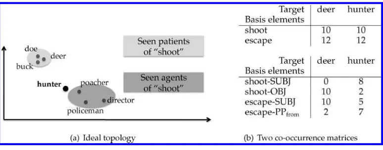
Figure 1

An idealized vector space for the plausibilities of (shoot,agent,hunter) and (shoot,patient,hunter).

fillers of the agent and patient position ofshoot, respectively. In order to judge whether a hunter is a plausible agent ofshoot, the vector space representation ofhunteris compared to the members of the exemplar cloud for the agent position—namely,poacher,policeman, and director. Due to the high average similarity of thehuntervector to these vectors, hunterwill be judged a fairly good agent ofshoot. Compare this with the result for the patient role:hunteris rather distant fromroe,deer, andbuck, and is therefore predicted to be a bad patient ofshoot. However, note thathunteris still more plausible as a patient ofshootthan, for example,director.

3.3 Formalization and Parameter Choice

Vector space models have been formalized by Lowe (2001) as tuples VS = (DTrans, Basis,sim,STrans), where Basis is a set of basis elements or dimensions, DTrans is a transformation of raw co-occurrence counts,simis a similarity measure, andSTransis a transformation of the whole space, typically dimensionality reduction. An additional parameter that becomes relevant for our use of vector spaces (cf. Equation [6]) is the weighting functionwtthat determines the contribution of each exemplar to the overall similarity. We discuss the parameters in turn and discuss our reasons for either explor-ing them or fixexplor-ing them.

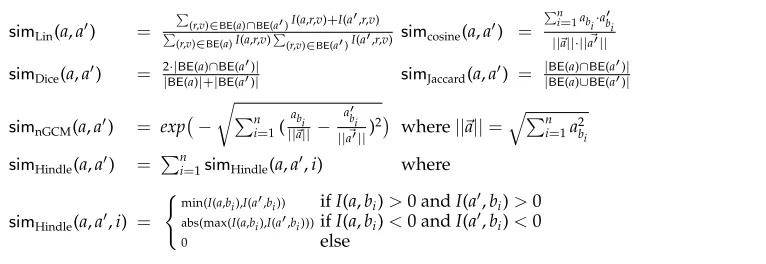
Table 2

Similarity measures explored in this article. Notation: We assumeBasis={b1,. . .,bn}. We writeI

for mutual information, andBE(a) for the set of basis elements that co-occur at least once witha.

simLin(a,a) =

(r,v)∈BE(a)∩BE(a)I(a,r,v)+I(a,r,v)

(r,v)∈BE(a)I(a,r,v)

(r,v)∈BE(a)I(a,r,v) simcosine(a,a _{) =}

n i=1a_bi·a_bi ||a||·||a||

sim_Dice(a,a) = 2_|BE·|BE_(a)(_|a₊)∩BE_|BE(₍a_a))|_| sim_Jaccard(a,a) = _||BE_BE(₍a_a)₎∩BE_∪BE((a_a)₎|_|

simnGCM(a,a) = exp

−

n

i=1( a

bi ||a||−

a

bi ||_a||)2

where||a||=n_i=1a2 bi

sim_Hindle(a,a) = n_i=1sim_Hindle(a,a,i) where

sim_Hindle(a,a,i) =

_min(I(a,b

i),I(a,bi)) ifI(a,bi)>0 andI(a,bi)>0

abs(max(I(a,b_i),I(a,b_i)))ifI(a,b_i)<0 andI(a,bi)<0

0 else

the resulting spaces gain the ability to distinguish between words likehunteranddeer, based on differences in typical occurrences in argument positions.

On the downside, dependency-based spaces are more expensive to compute than word-based spaces because they require a corpus with syntactic analysis. Thus, we explore both options. The word-based space records co-occurrences within a surface window of 10 (lemmatized) words.3 We refer to it as WORDSPACE. The dependency-based space, calledDEPSPACE, has basis elements consisting of a grammatical function

concatenated with a word, as in the bottom example in Figure 1(b) (Padó and Lapata 2007). Following earlier experiments on the representation of selectional preferences in word-dependency-relation spaces (Padó, Padó, and Erk 2007), we use a subject– object context specification that only considers co-occurrences between verbs and their subjects and direct objects.4_{In each case, we adopt the 2,000 most frequent context items} as basis elements.

Similarity measuresim.In principle, any similarity measure for vectors can be plugged into our model. Previous studies that compared similarity measures came to various conclusions about the usefulness of different measures. Cosine similarity is very popu-lar in Information Retrieval. Lee (1999) obtains good results for the Jaccard coefficient in pseudo-disambiguation. In the synonymy prediction task of Curran (2004), Dice emerged in first place. Padó and Lapata (2007) found good results with Lin’s measure for predominant word sense identification.

Because it is unclear whether the findings about best similarity measures general-ize to new tasks, we will investigate a range of similarity measures shown in Table 2: Cosine, the Dice and Jaccard coefficients, Hindle’s (1990) and Lin’s (1998) mutual information-based metrics, and an adaptation of Nosofsky’s (1986) Generalized Context Model (GCM), a model for exemplar-based similarity from psychology. The original GCM includes normalization by summed similarity over all classes of exemplars, which introduces competition between categories. Our version, which we callnGCM,instead normalizes by vector length to alleviate the influence of overall target frequency, but

3 We do not remove stop words for reasons of simplicity, as there is no unequivocal definition of this set, and we do not wish to remove potentially informative contexts.

4 This context specification is available assoonlyin the DependencyVectors software package

preserves the central idea that similarity decreases exponentially with distance (Shepard 1987).

All similarity measures from Table 2 are applicable to semantic spaces with arbitrary basis elements, with the exception of the Lin measure, whose definition applies only to dependency-based spaces. The reason is that it decomposes the basis elements into relation–word pairs (r,v). For semantic spaces with words as basis elements, the Lin measure can be adapted by omitting the random variabler(cf. Padó and Lapata 2007).

TransformationsDTrans andSTrans.Next, we come to transformations on counts and vec-tor spaces. Concerning the count transformationsDTrans, all counts are log-likelihood transformed (Dunning 1993), a standard procedure for word-based semantic space models which alleviates the problematic effects of the Zipfian distribution of lexical items, as proposed by Lowe (2001). As for transformations on the complete spaceSTrans, many studies do not perform dimensionality reduction at all. Others, like the LSA fam-ily of vector spaces (Landauer and Dumais 1997), regard it as a crucial ingredient. To gauge the impact ofSTrans, we compare unreduced spaces (2,000 dimensions) to 500-dimensional spaces created using Principal Component Analysis (PCA), a standard method for dimensionality reduction that identifies the directions of highest variance in a high-dimensional space.

Weight functions wt.Exemplar-based models are usually applied in conjunction with a function that can assign each exemplar an individual weight, which can be interpreted cognitively as degree of activation (Nosofsky 1986). We assess a small number of weight functions to investigate their importance within the EPP model. The first one,

UNI, assumes a uniform distribution,wtr,v(a)=1. The second one, FREQ, uses the co-occurrence frequency as weight,wtr,v(a)=freq(a,r,v), with the intuition that more fre-quent exemplars should be both more activated and more reliable. Finally, we consider a weight function that is an analogue of inverse document frequency in Information Retrieval. It weights words higher that occur with a smaller number of verb–role pairs: wtr,v(a)=log| a

Seenrv(a)|

|Seenrv(a)| , where we writeSeenrv(a) for the set of verb–role pairs (r,v) for which aoccurs as a headword.5 _{We abbreviate this weight function by DISCRfor} ‘discrimination’.

3.4 Discussion

Our EPP model can be seen as a straightforward implementation of the intuition to model selectional preference by generalizing from seen headwords to other, similar, words. We use vector space representations to judge the similarity of words, obtaining a completely corpus-driven model that does not require any additional resources and is very flexible. A complementary view on this model is as a generalization of traditional vector space models that represent semantic similarities between pairs of words. The

EPPmodel goes beyond this by computing similarity between a vector and a set of other

vectors. By instantiating the set with the vectors for seen headwords of some relationr, the similarity turns into a plausibility prediction that is specific to this relation.

Like other distributional models, the EPP model is applicable whenever corpus data are available; no lexical resource is required. Additionally, it does not require the headword observation step and the generalization step (cf. Section 1) to use the same

corpus.6 This allows us to work with a relatively small and deeply linguistically ana-lyzed corpus of seen headwords, the FrameNet corpus, while using a much bigger data set to generalize over seen headwords. It also allows us to make predictions for the potentially deeper relations annotated in the primary corpus, for example, semantic roles. We will investigate the potential of this setup in our Experiments 1 and 2.

As a distributional model, EPP avoids the two pitfalls of resource-based models. One is a coverage problem due to the limited size of the resource (see the task-based evaluation in Gildea and Jurafsky [2002]). For example, the semantic role–basedPADO ET AL. model resorts to class-based smoothing methods to improve coverage, which

EPPdoes not need. The other problem of resource-based models is that the shape of the WordNet hierarchy determines the generalizations that the models make. These are not always intuitive. For example, Resnik (1996) observes that (answer,obj,tragedy) receives a high preference becausetragedyin WordNet is a type of written communication, which is a preferred argument class ofanswer.

TheROOTH ET AL. model (Rooth et al. 1999) shares the resource independence of

EPP, but has complementary benefits and problems. Querying the probabilisticROOTH ET AL. model takes only constant time, whereas querying the exemplar-based EPP

model takes time linear in the number of seen arguments for the argument position. However, the ROOTH ET AL. model requires a dedicated training phase with a space

complexity linear in the total number of verbs and nouns, which can lead to practical problems for large corpora (cf. Section 5.1). The separation of similarity computation and headword observation inEPPalso gives the experimenter more fine-grained control over the types and sources of information in the model.

TheEPPmodel looks superficially similar to the model of Dagan, Lee, and Pereira (1999). However, they differ in the role of the similarity measure: The Dagan, Lee, and Pereira model computes a co-occurrence probability, and it uses similarity as a weight-ing scheme. The EPPmodel computes similarity (of a word to the typical fillers of an argument position), and its weighting schemes are separate from the similarity measure. The two models also differ in the kinds of items they consider as a basis for generaliza-tion (or smoothing): In computing the probability of seeing a wordw2afterw1, the sum in the Dagan, Lee, and Pereira model runs over all words that are similar tow1, whereas the sum in theEPPmodel runs over all words that have been seen as headwords in the argument position in question. Given that occurrence in an argument position is a form of co-occurrence, and similarity (in both models) is computed on the basis of vectors derived from co-occurrence counts, one could say that the sum in theEPP model runs

over words determined by first-order co-occurrence, whereas the sum in Dagan, Lee, and Pereira runs over words chosen through second-order co-occurrence (wherew1and w2are second-order co-occurring if they both tend to occur with the same wordsw3).

4. Design of the Experimental Evaluation

In this section, we give a high-level overview over the experiments and experimental settings we will use subsequently. Details will be provided in the following sections.

We evaluate the EPP model in three ways: We test the prediction of verbal selectional preference models with a pseudo-disambiguation task (Experiment 1). Then, we address the task of predicting human verb–argument plausibility ratings (Experiment 2). Finally, we investigate inverse selectional preferences—preferences of

nouns for the predicates that they co-occur with—again using pseudo-disambiguation (Experiment 3).

We compare theEPPmodel to models from the three model categories presented in Section 2:RESNIKas a hierarchical model;ROOTH ET AL. as a distributional model; and PADO ET AL. as a semantic role–based model. As both Brockmann and Lapata (2003)

and Padó (2007) have argued, no WordNet-based model systematically outperforms the others, and the RESNIKmodel shows the most consistent behavior across different scenarios. Among the distributional models, we chooseROOTH ET AL. as a model that performs soft clustering and thus shows a marked difference to theEPPmodel. To our knowledge, this is the first comparison of all three generalization paradigms: semantic hierarchy–based, distributional, and semantic role–based.7

As mentioned earlier, we employ two tasks to evaluate the four models: disambiguation and the prediction of human plausibility ratings. The pseudo-disambiguation task (Yarowsky 1993) has become a standard evaluation measure for selectional preference models (Dagan, Lee, and Pereira 1999; Rooth et al. 1999). Given a choice of two potential headwords, the task of a selectional preference model is to pick the more plausible one to fill a particular argument position of a given predicate. Pseudo-disambiguation can be viewed as a word sense disambiguation task in which the two potential headwords together form a “pseudo-word,” for exampleherb/struggle from the original wordsherb andstruggle. The task is to “disambiguate” the pseudo-word to the pseudo-word that fits better in the given context. It can also be viewed as an in vitro version of semantic role labeling and dependency parsing (depending on whether the relations are semantic roles or grammatical functions) (Zapirain, Agirre, and Màrquez 2009). In this case, the scenario is that of a sentence containing a predicate and two words that could potentially fill an argument position of that predicate, for example, the predicaterecommendwith the potential headwordsherbandstrugglefor the grammatical relation of direct object. The task is to decide which of the two potential headwords is better suited to fill the argument position.

Human plausibility ratings, on the other hand, make considerably more fine-grained distinctions than those occurring in pseudo-disambiguation tasks. Here, mod-els predict the exact human ratings for verb–argument–role triples. Ratings are collected to further control carefully selected experimental items for psycholinguistic studies (Trueswell, Tanenhaus, and Garnsey 1994; McRae, Spivey-Knowlton, and Tanenhaus 1998), or are solicited for corpus-derived triples specifically to create evaluation data for plausibility models (Brockmann and Lapata 2003; Padó 2007).

We contrast two different levels of semantic analysis for the predicates and argu-ment positions. In theSEM PRIMARYsetting, the predicates are FrameNet frames, each of them potentially instantiated by multiple different verbs. The argument positions in these settings are frame-semantic roles. This setting most closely matches the notion of selectional preferences as characterizations of semantic arguments of an event. In addition, we study theSYN PRIMARYsetting, where predicates are verbs, and argument positions are grammatical functions (subject and direct object). Viewing grammatical functions as shallow approximations of semantic roles, we can expect the selectional preference models for this setting to yield noisier estimates than in the SEM PRIMARY

setting. The two settings will differ only in the choice of primary corpus, but will use the same generalization corpus.

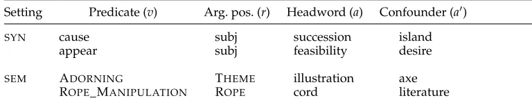
Table 3 illustrates the difference between the SEM PRIMARY setting and the SYN PRIMARYsetting on an example from a pseudo-disambiguation task: TheSEM PRIMARY

setting has predicates like the FrameNet frame (predicate sense) ADORNING, with the semantic role THEMEas argument position. In contrast, theSYN PRIMARY setting has

predicates that are verb lemmas, such ascause, and argument positions that are gram-matical functions (subj). In both settings, the two potential headwords (here called headword andconfounder, to be explained in more detail in the next section) to be distinguished in the pseudo-disambiguation task are noun lemmas.

The verb–dependency–headword tuples of the SYN PRIMARY setting yield much more coarse-grained and noisy characterizations of selectional preferences; however, they can be extracted from corpora with only syntactic annotation. We are therefore able to use the 100-million word BNC (Burnard 1995) as the primary corpus for this setting by parsing it with the Minipar dependency parser (Lin 1993). Minipar could parse almost all of the corpus, resulting in 6,005,130 parsed sentences.

For the SEM PRIMARY setting, we require a primary corpus with role-semantic annotation. We use the much smaller FrameNet corpus (Fillmore, Johnson, and Petruck 2003). FrameNet is a semantic lexicon for English that groups words in semantic classes called frames and lists fine-grained semantic argument roles for each frame. Ambiguity is expressed by membership of a word in multiple frames. Each frame is exemplified with annotated example sentences extracted from the BNC. The FrameNet release 1.2 comprises 131,582 annotated sentences (roughly three million words). To determine headwords of the semantic roles, the corpus was parsed using the Collins (1997) parser. As generalization corpus, we use the Minipar-parsed BNC in both settings. The ex-perimentation with two different primary corpora allows us to directly study the influ-ence of the disambiguation of predicates and the semantic characterization of argument positions on the performance of selectional preference models. Note, however, that the comparison is complicated by differences between the two corpora: The primary corpus for theSYN PRIMARYsetting is parsed automatically, which can introduce noise in the determination of predicates, grammatical functions, and headwords. The primary cor-pus for the SEM PRIMARY setting is manually annotated for semantics but is parsed automatically to determine headwords. This can introduce noise in the headwords, but not in the determination of predicates and semantic roles. Also, the primary corpus for theSYN PRIMARYsetting is much larger than the one used in theSEM PRIMARYsetting.

5. Experiment 1: Pseudo-Disambiguation

The first experiment uses a pseudo-disambiguation task to evaluate the models’ perfor-mance on modeling the plausibility of nouns as headwords of argument positions of verbal predicates.

Table 3

Pseudo-disambiguation items for theSYN PRIMARYsetting and theSEM PRIMARYsetting.

Setting Predicate (v) Arg. pos. (r) Headword (a) Confounder (a)

SYN cause subj succession island

appear subj feasibility desire

SEM ADORNING THEME illustration axe

Require: Some corpusT: a list of triples (v,r,a) of seen predicates, roles, and arguments. Require: Some corpusN: a list of noun lemmas, along with a functionfreqN :N→

that associates each nounn∈Nwith its corpus frequency.

1: Nmid={n∈N|freqN(n)≥30 andfreqN(n)≤3, 000}

2: We define a probability distributionpNover then∈NmidbypN(n)=freqN_mfreq(Nn()m)

3: conf ={ }# set of headword/confounder mappings, starts empty

4: AT={a|(v,r,a)∈T}# set of seen headwords 5: foreveryainATdo

6: choose a confoundera∈Nmidaccording topN 7: conf =conf ∪ {a→a}

8: end for

9: Return: conf

Figure 2

Algorithm for choosing confounders.

5.1 Setup

Task and data. In a data set of tuples (v,r,a) of a predicatev, argument positionr, and headworda, each tuple is paired with a confoundera. The task is to pick the original headword by comparing the tuples (v,r,a) and (v,r,a). Table 3 shows some examples.

We begin by collecting all triples (v,r,a) observed in the respective primary corpus. In the SYN PRIMARYsetting, this corresponds to all headwords observed in subject or direct object position of a verbal predicate in the BNC, and in theSEM PRIMARYsetting, to all nouns observed as headword of some semantic role in a frame introduced by a verb. From this set of triples (v,r,a) for a given primary corpus, we draw anevaluation samplethat is balanced by the corpus frequency of predicates and argument position. As test set, we choose 100 (v,r) pairs at random, drawing 20 pairs each from five fre-quency bands: 50–100 occurrences; 100–200 occurrences; 200–500; 500–1,000; and more than 1,000 occurrences. For any chosen predicate–relation pair, we sample triples (v,r,a) equally from six frequency bands of arguments a: 1–50 occurrences; 50–100; 100–200; 200–500; 500-1,000; and more than 1,000 occurrences. These evaluation samples contain a total of 213,929 (SYN) and 65,902 (SEM) tuples.

Next, we pair each headword with a confounder sampled from the primary corpus as described in Figure 2.8_{In the literature, there have been two different approaches to} choosing confounders for pseudo-disambiguation tasks: The first approach, used by Dagan, Lee, and Pereira (1999), chooses confounders to match the headword a in frequency. The second approach, used in Rooth et al. (1999), sets the probability that a word is drawn as a confounder to its relative frequency. The advantage and dis-advantage of the first approach is that it largely eliminates the frequency bias that is a general problem of vector space-based approaches. This is an advantage in that it allows the generalization achieved by the model to be evaluated without any distortion from frequency bias. It is a disadvantage in that in any practical application making use of selectional preferences, the data will not be frequency-balanced. For example, selectional preferences could be used by a dependency parser to decide which word in the sentence to link to a given verb via a subject edge, or selectional preferences could

be used by a semantic role labeler to decide which constituent is the overall best filler for the AGENTrole for a given predicate. In such cases, it does not appear warranted to assume that the frequencies of different headword candidates are balanced. We choose the second option for our experiments, using relative corpus frequency to approximate the probability of encountering different headword candidates.

Training of models.As stated earlier, we evaluate all models in theSYN PRIMARYsetting

and theSEM PRIMARYsetting. In all experiments herein, we perform two 2-fold

cross-validations runs. In each run, we randomly split the respective (SYNorSEM) evaluation sample into a training and a test set at the token level. Figure 3 describes the experimen-tal procedure in pseudo-code.

TheEPP,RESNIK, andPADO ET AL. models are trained on the training split of the evaluation sample. TheEPPmodel additionally uses the BNC as generalization corpus in both the SYN PRIMARY setting and the SEM PRIMARY setting. This generalization corpus is used to compute either a WORDSPACE or a DEPSPACE vector space, as discussed in Section 3.3. For theROOTH ET AL. model, we had to employ a frequency

Require: A setFormalismsof formalisms to test

Require: A primary corpus T: a list of triples (v,r,a) of seen predicates, argument positions, and arguments, along with a functionfreqT:T→that associates each

triple (v,r,a)∈Twith its corpus frequency

Require: A mappingconf :Lemmas→Lemmasof headwords to confounders such that

{a|(v,r,a)∈T} ⊆Domain(conf)

1: eval_results={ } 2: forsplitno in 1:2do

3: # prepare two independent splits

4: half1={ },half2={ }# mappings from headwords to counts

5: foreach tupletinTdo

6: # decide how many occurrences of t to put in half1, half2by drawing from the binomial distribution

7: Samplek∼B(freqT(t), 0.5)

8: half1=half1∪ {t→k},half2=half2∪ {t→freqT(t)−k} 9: end for

10: splits={(half1,half2), (half2,half1)}

11: for(ftrain,ftest) insplitsdo

12: foreach formalismFinFormalismsdo

13: train a modelmFaccording to formalismFusing the training set defined by the frequency functionftrain.

14: foreach tuple (v,r,a) inTdo

15: fori in 1:ftest(v,r,a)do

16: Evaluate the performance ofmFon the tuple (v,r,a,conf(a)) and add the result toeval_results

17: end for

18: end for

19: end for

20: end for

21: end for

22: Return: eval_results

Figure 3

cutoff of five in theSYN PRIMARYsetting to reduce the amount of training data due to memory limitations. ThePADO ET AL. model is only used in theSEM PRIMARYsetting: FrameNet is an integral part of this model, and it cannot be used in a syntax-only setting without major changes. For details on training, see Section 2.4. Note that no verb classes had to be induced from the data, because the predicates v are already instantiated by verb classes, namely, FrameNet frames (see Table 3).

Finally, we report three baselines. The first baseline,headword frequency(HW), is very simple. It decides between the headword aand the confounderaby comparing the frequenciesf(a) andf(a). The second, more informed, baseline istriple frequency (TRIPLE). It votes foraiff(v,r,a)>f(v,r,a), and vice versa. The third baseline, abigram language model(LM), was constructed by training a 2-gram language model from the large English ukWAC Web corpus (Baroni et al. 2009) using the SRILM toolkit (Stolcke 2002) with default Good–Turing smoothing. We retained only verbs, nouns, adjectives, and adverbs in order to maximize the proximity between verbs and their subjects and objects. We defined the preference score for verb–subject triples as the probability of the sequence av, that is, Pref(v,subj,a)=P(v|a). Conversely, the preference score for verb– object triples was defined as the probability of the sequenceva, that is,Pref(v,obj,a)=

P(a|v). Again, the model comparesPref(v,r,a) andPref(v,r,a) to make its decision.

Evaluation.For all models, we report two evaluation figures. One iscoverage: A tuple is covered if the model assigns some preference toboth aanda, and the preferences are not equal. The second iserror rate, which is the relative frequency, among allcovered tuples, of instances where the confounder was at least equally preferred. Both coverage and error rate are averages over the 2 x 2 cross-validation runs in each setting.

We determine the statistical significance of differences between error rates using bootstrap resampling (Efron and Tibshirani 1994). This procedure samples correspond-ing model predictions with replacement from the set of predictions made by the models to be compared and computes the difference in error rates. On the basis of n such samples (n= 1,000), the empirical 95% confidence interval for the difference in strength on the basis of all observed differences is computed. If the interval includes 0, the difference is not statistically significant.

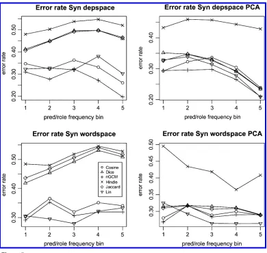
5.2SYN PRIMARYSetting: Results

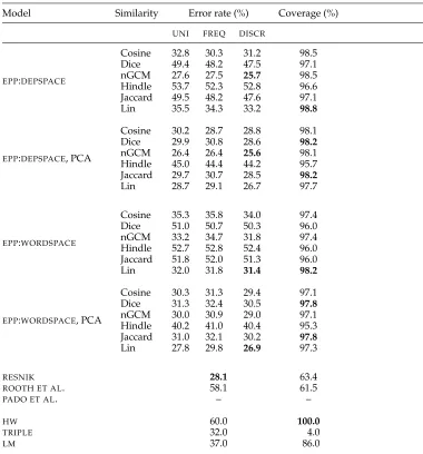
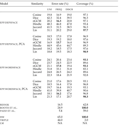
Table 4 shows the results for the SYN PRIMARY setting. The overall best error rate is

achieved by a variant of the EPP model, with the RESNIK model coming in second

(the performance difference is significant at the 0.05 level). TheEPPvariants also show near-perfect coverage, whereas the RESNIKmodel delivers results only for 63% of the data points. We found a very high error rate and a comparatively low coverage for

ROOTH ET AL., which most likely stems from the data pruning necessary to reduce the training data (compare the subsequent results in the SEM PRIMARYsetting). ThePADO ET AL. model was not tested in theSEM PRIMARY setting, because it requires semantic role annotation. TheHWbaseline is somewhat below chance (50%), which is an effect of our by-token sampling procedure, according to which confounders often have higher corpus frequencies than the real arguments. TheTRIPLEbaseline has a better error rate than theLMbaseline, but has very low coverage. Both theRESNIKand theEPPmodels outperform the baselines in terms of error rate. That they outperform the TRIPLE

Table 4

SYN PRIMARYsetting: Pseudo-disambiguation results for different weighting schemes.

Model Similarity Error rate (%) Coverage (%)

UNI FREQ DISCR

EPP:DEPSPACE

Cosine 32.8 30.3 31.2 98.5

Dice 49.4 48.2 47.5 97.1

nGCM 27.6 27.5 25.7 98.5

Hindle 53.7 52.3 52.8 96.6 Jaccard 49.5 48.2 47.6 97.1

Lin 35.5 34.3 33.2 98.8

EPP:DEPSPACE, PCA

Cosine 30.2 28.7 28.8 98.1

Dice 29.9 30.8 28.6 98.2

nGCM 26.4 26.4 25.6 98.1

Hindle 45.0 44.4 44.2 95.7 Jaccard 29.7 30.7 28.5 98.2

Lin 28.7 29.1 26.7 97.7

EPP:WORDSPACE

Cosine 35.3 35.8 34.0 97.4

Dice 51.0 50.7 50.3 96.0

nGCM 33.2 34.7 31.8 97.4

Hindle 52.7 52.8 52.4 96.0 Jaccard 51.8 52.0 51.3 96.0

Lin 32.0 31.8 31.4 98.2

EPP:WORDSPACE, PCA

Cosine 30.3 31.3 29.4 97.1

Dice 31.3 32.4 30.5 97.8

nGCM 30.0 30.9 29.0 97.1

Hindle 40.2 41.0 40.4 95.3 Jaccard 31.0 32.1 30.2 97.8

Lin 27.8 29.8 26.9 97.3

RESNIK 28.1 63.4

ROOTH ET AL. 58.1 61.5

PADO ET AL. – –

HW 60.0 100.0

TRIPLE 32.0 4.0

LM 37.0 86.0

are dissimilar from other seen headwords, which allows RESNIK and EPP to identify them as confounders in spite of their higher co-occurrence frequency.

The difference between UNI and DISCR is significant throughout; the difference betweenFREQandDISCRis less uniform. InDEPSPACE, the difference between the best measure with and without PCA (nGCM in both cases) is not significant; inWORDSPACE, the difference between the best measure with and without PCA (Lin in both cases) is significant (p≤0.01).

For bothWORDSPACEs andDEPSPACEs without PCA, the similarity measures divide into two distinct groups: Lin, nGCM, and Cosine on the one hand and Jaccard, Dice, and Hindle on the other, with a significant difference in performance between the groups (p ≤0.01). The use of dimensionality reduction through PCA improves performance for all similarity measures, in WORDSPACEas well as DEPSPACE. The improvement is especially marked for the Dice and Jaccard measures, which perform at the level of a random baseline for unreduced spaces. We assume that these set intersection-based measures benefit from the independent dimensions that PCA produces. For the simi-larity measures with best performance, the improvement through PCA is less marked. Thus, PCA-reduced spaces show more similar error rates across similarity measures. After PCA, only nGCM and Lin still significantly (p ≤ 0.01) outperform the others in DEPSPACE, and inWORDSPACE, Lin is the only measure that performs significantly differently from the rest (p≤0.01).

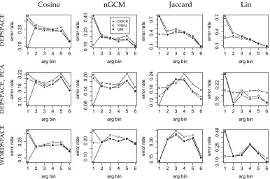
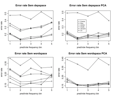
As arguments are sampled from six frequency bins, we can inspect the effect of argument frequency on error rate. Figure 4 examines the performance of theEPPmodel

with different similarity measures and weighting schemes by argument frequency bins (cf. the subsectionTask and Datain Section 5). We find that the overall best weighting scheme, DISCR, also works best for all except the highest argument frequency bin. In theDEPSPACEsetting (upper row), all similarity measures show a frequency bias in that

Figure 4

Figure 5

SYN PRIMARYsetting: Error rate bypredicatefrequency bin:DISCRweighting. Bins: 1 = 50–100; 2 = 100–200; 3 = 200–500; 4 = 500–1,000; 5 > 1,000.

error rate is lower for more frequent arguments, but this bias is much less pronounced in Cosine and nGCM than in the other measures, with error rates varying between 45% and 25% rather than 80% and 20%. (Dice and Hindle, not shown here, exhibit similar behavior to Jaccard.) In PCA-transformedDEPSPACE(middle row), this frequency bias largely disappears for all similarity measures. InWORDSPACE(bottom row), although there is again a frequency bias in all similarity measures, Lin now joins Cosine and nGCM in being much less biased than Jaccard, Dice, and Hindle. For WORDSPACE

with PCA-transformation, not shown here, the curves resemble those ofDEPSPACEwith PCA-transformation.

WORDSPACE. It seems that in the sparser DEPSPACE, models can still profit from the additional seen headwords in the highest predicate frequency bins, whereas in the less sparse but noisier WORDSPACE, the added noise is stronger than the added signal in the highest predicate frequency bins. For the lowest predicate frequency bins, the best results inWORDSPACEare better than those inDEPSPACE.

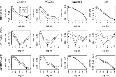
5.3SEM PRIMARYSetting: Results

Table 5 shows the results for theSEM PRIMARYsetting, where we predict head words for pairs of a frame (predicate sense) and semantic role. In comparison to theSYN PRIMARY

setting (Table 4), error rates are lower across the board. The difference for theEPPmodels is on average around 10%.

Table 5

SEM PRIMARYsetting: Pseudo-disambiguation results for different weighting schemes.

Model Similarity Error rate (%) Coverage (%)

UNI FREQ DISCR

EPP:DEPSPACE

Cosine 19.8 16.9 19.0 97.1

Dice 42.3 32.4 39.5 96.3

nGCM 20.2 16.3 20.8 97.1

Hindle 48.3 46.8 47.8 93.4 Jaccard 41.5 31.5 38.5 96.3

Lin 31.1 20.2 29.0 97.7

EPP:DEPSPACE, PCA

Cosine 18.5 17.0 17.8 96.9

Dice 19.3 19.2 18.0 97.6

nGCM 16.9 15.7 16.4 96.9

Hindle 44.9 45.6 44.7 89.3 Jaccard 18.2 18.5 17.5 97.6

Lin 18.8 19.5 18.3 98.9

EPP:WORDSPACE

Cosine 24.1 20.4 23.4 93.1

Dice 23.7 24.5 22.5 89.6

nGCM 21.1 17.8 19.4 93.1

Hindle 31.8 33.1 31.8 83.1 Jaccard 24.8 26.5 24.2 89.6

Lin 22.3 18.4 21.9 92.8

EPP:WORDSPACE, PCA

Cosine 21.0 17.6 20.5 93.1

Dice 18.5 16.4 17.8 96.8

nGCM 19.7 16.4 19.3 93.1

Hindle 41.0 39.8 40.7 90.6 Jaccard 18.1 16.2 17.6 96.8

Lin 21.3 17.1 20.7 98.3

RESNIK 16.5 62.8

ROOTH ET AL. 24.9 100.0

PADO ET AL. 7.1 59.0

HW 65.0 100.0

TRIPLE 44.0 2.0

The error rate of thePADO ET AL. model, at 7%, is the best by a large margin. We attribute this to the extensive generalization mechanisms that the model uses, which draw on an array of lexical–semantic resources. However, with a coverage of 59%, the model is still unable to make predictions for many of the test items. Error rates for theRESNIKand theEPPmodels are comparable, at 16.5% forRESNIKand 15.7% for

the best EPP variant. The two models differ sharply in coverage, however: 62.8% for

RESNIK, consistent with the findings of Gildea and Jurafsky (2002), and between 90% and 98% forEPPvariants. TheRESNIKmodel also profits from the presence of semantic disambiguation in the SEM PRIMARY setting (in the SYN PRIMARY setting its error rate was 28%), which underlines the substantial impact that properties of the training data have on semantic hierarchy–based models of selectional preferences. ROOTH ET AL. now has perfect coverage, affirming our assumption that the very bad results of the ROOTH ET AL. model in the SYN PRIMARYsetting were an artifact of the data sampling necessary for that data set. Although its error rate of 24.9% is a substantial improvement over all baselines, the EPP model achieves error rates that are up to 9 points lower at a comparable coverage. Among the baselines,HWshows that here, as in theSYN PRIMARYsetting, arguments have some tendency of having lower frequency than the confounders. The TRIPLE baseline shows near-random performance, at very low coverage, a result of the very small size of the corpus. Because there is no large corpus with frame-semantic roles, nor is the annotation easily linearizable, we could not compute aLMbaseline in theSEM PRIMARYsetting.

AmongEPPmodels, theDEPSPACEs andWORDSPACEs perform comparably, with a non-significant advantage for DEPSPACE among the best models. Overall error rates show the same clear divide between the three high-performing similarity measures (Cosine, nGCM, and Lin) and the three weaker ones (Dice, Jaccard, and Hindle). Di-mensionality reduction again dramatically improves the weaker models, with Jaccard yielding the best result for the PCA-reduced WORDSPACE.9 _{Whereas all best} parame-trizations in theSYN PRIMARYsetting usedDISCRweighting, it is nowFREQweighting that yields the best results.

Figure 6 again analyzes the influence of argument frequency on performance by showing the performance of different variants of the EPP model over six argument frequency bins. The upper row shows DEPSPACE without dimensionality reduction. Note thatFREQweighting now works especially well for the lowest argument frequency bin, much better than DISCR and PLAIN. This is the opposite of what we saw for the SYN PRIMARYsetting in Figure 4. With DISCR and PLAINweighting, Jaccard and Lin

again have noticeable problems with the lowest argument frequency bins—as in theSYN PRIMARYsetting—but not with FREQ weighting. WithDEPSPACE and dimensionality reduction (middle row), we get error rates of≤26% for all settings and all frequency bins. On the lowest frequency bin, we again see a large advantage ofFREQweighting over the two other weighting schemes. The bottom row shows WORDSPACE without dimensionality reduction. Note that there is much less variation in error rates across frequency bins here than in unreducedDEPSPACE.

Figure 7 charts error rate by predicate frequency bin, showing FREQ weighting only, as this showed the best results on this data set. The figure clearly illustrates the divide between the top and the bottom three similarity measures inDEPSPACE, as well as the disappearance of this divide for both PCA settings. In unreducedWORDSPACE,

the divide is not as clearly visible. The figure also indicates a slight tendency for error rates to rise for the lowest-frequency as well as the highest-frequency predicates, across all spaces.

5.4 Discussion

The resource-based approaches that we tested,RESNIKandPADO ET AL., show superior performance when they have coverage (which coincides with findings in other lexical semantics tasks that supervised data, when available, always increases performance), but showed low coverage, at most 63% (RESNIK,SYN PRIMARYsetting). TheEPPmodel achieves near-perfect coverage at good error rates: In the SYN PRIMARY setting, the

RESNIKmodel achieved an error rate of 28%, and the bestEPP variant was at 26%. In the SEM PRIMARY setting, error rates were 7% for the PADO ET AL. model, 16.5% for the RESNIKmodel, and 16% for the best EPPvariant. Comparing the EPP and ROOTH ET AL. models in theSEM PRIMARYsetting, we find that the use of an additional

gen-eralization corpus in theEPPmodel seems to offset any advantages introduced by the

joint clustering of predicates and arguments.

The difference in model performance on the two primary corpora (SYNand SEM) is striking. Even though the FrameNet corpus is smaller and a sparse data prob-lem might be expected, models perform at considerably lower error rates in the SEM PRIMARY setting than when the primary corpus is the larger BNC. This underscores the point that selectional preferences belong to a predicatesenserather than a predicate lemma, and that they describe the semantics of fillers of semantic roles rather than of

Figure 6

Figure 7

SEM PRIMARYsetting: Error rate bypredicatefrequency bin:FREQweighting. Bins: 1 = 50–100; 2 = 100–200; 3 = 200–500; 4 = 500–1,000; 5 > 1,000.

syntactic dependents (recall that in this setting, we predict head words for pairs of a predicate sense and semantic role). In theSEM PRIMARYsetting, the data is cleaner, so it is expected that seen headwords of an argument position will be more semantically uniform. This has a strong influence on model performance. Another factor contributing to the difference in performance between the two data sets may be that the primary corpus in theSYN PRIMARYsetting is parsed automatically, whereas manual annotation

is available in the FrameNet corpus. However, although this manual annotation iden-tifies predicate senses, role headwords are still determined through automatic parsing. The division of the training data into a primary and a secondary corpus allows us to successfully use FrameNet as the basis for semantic space–based similarity estimates despite the fact that this corpus alone would be too small to sustain the construction of a robust space.

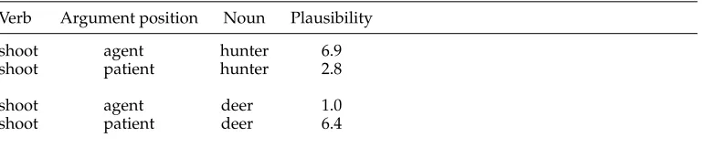
Table 6

Verb–argument position–noun triples with plausibility judgments on a 7-point scale (McRae et al., 1998).

Verb Argument position Noun Plausibility

shoot agent hunter 6.9

shoot patient hunter 2.8

shoot agent deer 1.0

shoot patient deer 6.4

theSYN PRIMARYsetting, as well as in allSEMconditions except reducedWORDSPACE.

The Lin measure seems to work well with noisier data: It is the bestEPP model when using WORDSPACE in the SYN PRIMARY setting. Cosine, although never showing the top performance, is among the best models in any setting. Although dimensionality reduction only improves the overall error rates of the best models by a few points, it has two important consequences: First, dimensionality reduction reduces dependence of the results on the exact similarity measure chosen, as all measures except Hindle show nearly indistinguishable error rates on reduced spaces (Figures 5 and 7). Second, low-frequency arguments profit by a huge margin when PCA is used (Figures 4 and 6). Among weighting schemes, DISCRweighting seems to be most useful when the data is sparse but somewhat noisy (as is the case in the lower argument frequency bins in theSYN PRIMARY setting). Frequency weighting seems to work best when the data is either not sparse (as in the highest argument frequency bin in theSYN PRIMARYsetting) or very clean but sparse (as in the lowest argument frequency bin in theSEM PRIMARY

setting). A comparison of the two vector spaces, DEPSPACE and WORDSPACE, shows

no clear winner. When the collections of seen headwords are noisier, as they are in the

SYN PRIMARY setting, DEPSPACE, with its more aggressive filtering, yields the better results. Sets of headwords collected by predicate sense, as in theSEM PRIMARYsetting, are sparser but cleaner, andWORDSPACEshows lower error rates.

6. Experiment 2: Human Plausibility Judgments

Experimental psycholinguistics affords a second perspective on selectional preferences: The plausibility of verb–argument pairs has been shown to have an important effect on human sentence processing (e.g., Trueswell, Tanenhaus, and Gransey 1994; Garnsey et al. 1997; McRae, Spivey-Knowlton, and Tanenhaus 1998). In these studies, plausibility was operationalized as the thematic fit or selectional preference between a verb and its argument in a specific argument position. Models of human sentence processing there-fore need selectional preference models (Padó, Crocker, and Keller 2009). Conversely, psycholinguistic plausibility judgments can be used to evaluate computational models of selectional preferences.

6.1 Experimental Materials