84
©IJRASET: All Rights are Reserved
Object Classification with Classical Linear
Discriminant Analysis and Robust Linear
Discriminant Analysis
Justin Eduardo Simarmata1, Sutarman2, Mardiningsih3 1, 2, 3
Faculty of Mathematics and Science, University of Sumatera Utara
Abstract: Discriminant analysis is one of multivariate analysis with dependency method. Discriminant analysis is a multivariate analysis that aims to classify observations based on several independent variables that are non-categorical and categorical dependent variables. Discriminant analysis requires the assumption of the normal multivariate distribution and the homogeneity of the variance-covariance matrix. Classical linear discriminant analysis and linear robust discriminant analysis can be applied to classify objects. The classification is based on 10 indicators of district/city poverty level in North Sumatra province, 10 indicators are as independent variable and low poverty classification and high poverty classification as dependent variable. The linear robust discriminant model classifies the object more precisely than the classic linear discriminant model. This can be seen from the total proportion of classification mistakes of 6%, less than the total proportion of classical linear discriminant classifier error classification of 21.2%. This is due to the large number of outlays in the district/city poverty data in North Sumatra. Keywords: multivariate analysis, the classical linear discriminant analysis, robust
I. INTRODUCTION
Multivariate analysis is a statistical analysis that is imposed on the data that consists of many variables and intercorrelated variables. Multivariate data not only consists of one variable, but may consist of more than one variable. Multivariate analysis is a statistical technique used to understand the data structures in high dimensions. The variables are related to one another. There in lies the difference between multivariable and multivariate analyzes. Multivariate inevitably involves a multivariable but not vice versa. Multivariable mutually correlated which is said multivariate.
Discriminant analysis is a multivariate analysis that aims to classify observations based on several independent variables that are non-categorical and categorical dependent variables. Discriminant analysis requires the assumption of multivariate normal distribution and homogeneity of variance-covariance matrix. In the application of discriminant analysis to consider the outliers in the data. Therefore, the average vector and variance-covariance matrices are predicted by the robust minimum covariance determinant (MCD) method of the outliers.
Seeing the many methods of grouping objects that exist to encourage researchers to compare the methods with each other to determine the most accurate method of classifying an object. The model will be established in this study is the classical linear discriminant analysis and linear discriminant analysis robust. The second analysis was chosen as the object classification of the most widely used both theoretically and practically. The analysis is also a kind of analysis of the most widely developed by many researchers because it has a level of accuracy and precision in classifying an object that is higher than any other method types. This stuy aims to classify the data rate of poverty districts/cities in North Sumatra by linear discriminant analysis classical and discriminant analysis robust, obtain the classification of objects into a group with the method of linear discriminant analysis classical and robust and compare results of the classification method of linear discriminant analysis classic with robust discriminant analysis to obtain the best results based on wrong classification of the minimum.
II. DISCRIMINANT ANALYSIS
85
©IJRASET: All Rights are Reserved
that is able to distinguish an object enter the group in which categories.
A. Multivariate Normality Test
To test the normality of multiple variables is to find the value of squared distance for each observation that is: = ( − ) ( − )
B. The Variance Covariance Matrix Similarity Test
To test the variance covariance matrix similarity group I (S1) and group II (S2) used a hypothesis:
H0 : S1 = S2, the variance matrix of group covariance is relatively the same
H1 : S1 ≠ S2, the matrix of covariance variance of the group is significantly different
accept H0, which means the matrix of covariance variance is the same if:
≤ ∝. ( ) ( )
with:
=−2( −C ) ∑ ln |S |− ln | |∑
with:
= – 1
S = ∑
∑
C1 = ∑ − ∑ ( )(
)
C. Variance Difference Variance Testing
The test statistic used to test the average between groups is statistic F with the hypothesis: H0 : = = . . . = , means the mean between groups is the same (no difference)
H1 : ≠ ≠ . . . ≠ , means there is an average difference between groups
= Level of Significance
Critical areas : rejected H0, jika Fcount > Ftable
Ftable = ∝( ; )
db1 = k – 1
db2 = (n - k) = (n1 - 1) + (n2 - 1)
D. Outlier Detection
Outlier is an observation that is far (extreme) from other observations. An observation xi is detected as an outlier if its mahalanobis
distance is as follows:
= ( − ) ( − )> .(∝)
E. Function of Discriminant Analysis
The discriminant function is a linear combination of variables belonging to groups to be classified. In the i-nth observed data (i = 1, 2, ... , n) consisting of variables are X1, X2, . . . , Xj. The observational data can be presented in the following matrix form.
Table 1. Observational Data Matrix
Variables X1 X2 ⋯ Xj
Observation data X11 X12 ⋯ X1j
X21 X22 ⋯ X2j
⋮ ⋮ ⋮
Xn1 Xn2 ⋯ Xnj
86
©IJRASET: All Rights are Reserved
Sjj =
∑ ∑
( )
For the variables Xi and Xj where i ≠ j there is covariance, given the symbol Sij which can be calculated by the following formula:
Sij =
∑ ∑ ∑
( )
Variance and covariance are arranged in a matrix called the variance-covariance matrix with the symbol S:
S =
⎣ ⎢ ⎢
⎡S S ⋯ S
S S ⋯ S
⋮ S ⋮ S ⋯ ⋯ ⋮ S ⎦ ⎥ ⎥ ⎤
The variables in each group can be written in column vector form as follows.
= ⋮ and = ⋮
declares the variable X to j in group to 1 declares the X variable to j in group to 2
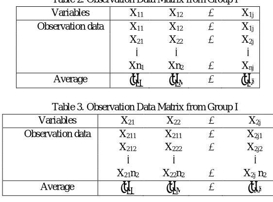
From each n1-sized group of the 1st and n2-sized groups of the 2nd group. Observation data will be in the form of a matrix that
[image:3.612.164.445.341.549.2]looks like the following.
Table 2. Observation Data Matrix from Group I
Variables X11 X12 ⋯ X1j
Observation data X11 X12 ⋯ X1j
X21 X22 ⋯ X2j
⋮ ⋮ ⋮
Xn1 Xn2 ⋯ Xnj
Average ⋯
Table 3. Observation Data Matrix from Group I
Variables X21 X22 ⋯ X2j
Observation data X211 X211 ⋯ X2j1
X212 X222 ⋯ X2j2
⋮ ⋮ ⋮
X21n2 X22n2 ⋯ X2j n2
Average ⋯
The results of this observation will produce the mean for each variable formed in vector form can be written:
= ⎣ ⎢ ⎢ ⎡ ⋮ ⎦ ⎥ ⎥ ⎤
and =
⎣ ⎢ ⎢ ⎡ ⋮ ⎦ ⎥ ⎥ ⎤ where:
X1jn1 declares variable X to j in group to 1 of size n1
X2jn2 declares variable X to j in group 2 that is n2 sized
states the average of variables to j in group 1 states the average of variables to j in group 2
87
©IJRASET: All Rights are Reserved
S1 =
⎣ ⎢ ⎢
⎡S S ⋯ S
S S ⋯ S
⋮ S ⋮ S ⋯ ⋯ ⋮ S ⎦ ⎥ ⎥ ⎤
and S2 =
⎣ ⎢ ⎢
⎡S S ⋯ S
S S ⋯ S
⋮ S ⋮ S ⋯ ⋯ ⋮ S ⎦ ⎥ ⎥ ⎤
where : S1 = matrix of covariance variance of group 1
S2 = matrix of covariance variance of group 2
Both matrices of this variance-covariance matrix can be calculated by the combined variance-covariance matrix, given the symbol S with the formula:
S = ( ) ( )
This combined variance-covariance matrix has an inverse, .
Given the mean vectors and and also the combined variance-covariance matrix S, the discriminant function formula is obtained:
Y = ( − ) .X
F. Robust Method
To overcome the existence of the pencil then used Minimum Covariance Determinant (MCD) estimator for μ and Σ which allegedly
by ̅ and S is
̅ = ∑
∑ and S =
∑ ( ̅ ) ( ̅ )
∑
thus, the discriminant score equation for RLDA becomes:
( ) = ̅ S − ̅ S ̅ + ln( ). = 1.2. … .
and the discriminant score equation for RQDA becomes:
( ) =− ln|S | − ( − ̅ ) S ( − ̅ ) + ln( ). = 1.2. … .
an observation x will be included in a group of k if the discriminant score: ( ) = maximum from ( ). ( ) … ( )
G. Apparent Error Rate (APER)
APER value can be calculated by:
APER =
where:
= the number of observations of group 1 were incorrectly classified as group 2 = the number of observations from group 2 were incorrectly classified as group 1
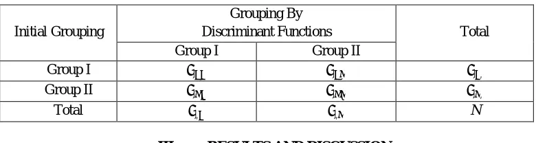
[image:4.612.112.502.572.676.2]H. The accuracy Grouping Discriminant Function
Table 4. Evaluation of Discriminant Functions
Initial Grouping
Grouping By
Discriminant Functions Total
Group I Group II
Group I ,
Group II ,
Total , , N
III. RESULTS AND DISCUSSION
88
©IJRASET: All Rights are Reserved
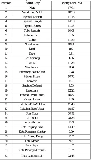
[image:5.612.149.466.112.668.2]District/Municipality Poverty Rate Data in North Sumatra:
Table 5. Poverty Rate of regencies/cities data in North Sumatra
Number District /City Poverty Level (%)
1 Nias 17.64
2 Mandailing Natal 10.98
3 Tapanuli Selatan 11.15
4 Tapanuli Tengah 14.58
5 Tapanuli Utara 11.25
6 Toba Samosir 10.08
7 Labuhan Batu 8.95
8 Asahan 11.86
9 Simalungun 10.81
10 Dairi 8.9
11 Karo 9.81
12 Deli Serdang 4.86
13 Langkat 11.36
14 Nias Selatan 18.6
15 Humbang Hasundutan 9.78
16 Pakpak Bharat 10.72
17 Samosir 14.4
18 Serdang Bedagai 9.53
19 Batu Bara 12.24
20 Padang Lawas Utara 10.87
21 Padang Lawas 8.69
22 Labuhan Batu Selatan 11.49
23 Labuhan Batu Utara 10.97
24 Nias Utara 30.92
25 Nias Barat 28.36
26 Kota Sibolga 13.3
27 Kota Tanjung Balai 14.49
28 Kota Pematang Siantar 9.99
29 Kota Tebing Tinggi 11.7
30 Kota Medan 9.3
31 Kota Binjai 6.67
32 Kota Padangsidimpuan 8.32
33 Kota Gunungsitoli 23.43
89
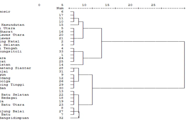
[image:6.612.143.503.75.308.2]©IJRASET: All Rights are Reserved
Figure 1. Cluster Hierarchical Cluster Analysis
A. Assumption Testing Discriminant Analysis 1) Multivariate Normal Test
Hypothesis
H0 : Educational data resolved at primary, junior, secondary, non-working, working in the informal sector, working in the formal
sector, users of contraceptives, the percentage of under-fives immunized, households of water users and households own toilet / shared normal multivariate.
H1 : Educational data resolved at primary, junior, senior secondary, unemployed, informal sector, working in the formal sector,
contraceptive users, the percentage of immunized toddlers, households of water users, and households own / shared toxic normal multivariate.
Level of significance (∝) = 0.05 Statistics Count:
p-value= 0.985 Testing Criteria:
H0 rejected if p-value ≤∝
Decision :
H0 accepted because p-value = 0.985
B. The Similarity Covariance Matrix Variants Test 1) Hypothesis
H0 : the covariance matrix of the high poverty status group and the low status group of poverty is the same.
H1 : the covariance matrix of the high poverty status group and the low status group of poverty is different.
Level of significance (∝) = 0.05 Statistics Count :
MC-1 = 0.08
Sig. = 0.00 Testing Criteria : H0 rejected if Sig. ≤∝
Decision :
90
©IJRASET: All Rights are Reserved
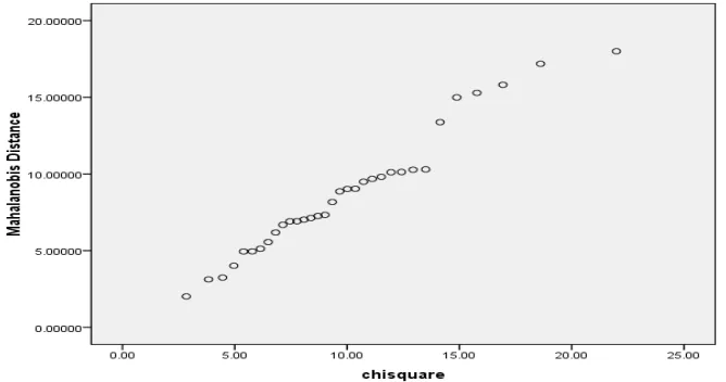
C. Outlier
[image:7.612.145.479.132.308.2]The outlier is a datum that deviates very far from the other datum in a sample or collection of datum. Scatter plot indicator Poverty districts / municipal ProvinsI of North Sumatra by using SPSS obtained:
Figure 2. Plot indicators that spread Poverty districts/cities of North Sumatra Province
D. Variable Selection Free
Based on the results of the selection of independent variables using SPSS, the independent variables that influence in determining the status of poverty level of regencies/cities in North Sumatra are variables X1, X2, X3, X4, X6, X7, X8, X9, and X10.
E. Classical Linear Discriminant Analysis
The discriminant parameter of discriminant function in classical linear discriminant analysis is done by finding ̅ and S which is the average vector and covariance matrix of the data. Based on calculations using standardized data, the average vector and covariance matrices are then converted, so that the classic linear discriminant function is obtained:
Y = 41,13131X1 - 4810,25X2 - 4771,78X3 - 5,94152X4 - 2080106X6 + 1683,34X7 - 13,0409X8 + 714,8802X9 + 4093,957X10.
Table 6. Classification results of the classic linear discriminant model for 33 data
Initial Grouping
Grouping By
Discriminant Functions Total
Group I Group II
Group I 14 3 17
Group II 4 12 16
Total 18 15 33
Table 6 explains that many objects classified appropriately for linear discriminant models in 33 regency/city data are as many as 26 objects and many objects are misclassified as many as 7 objects. Based on APER value, the total proportion of classical linear discriminant error is 21.2%, so classical linear discriminant classification is 78.8%.
F. Robust Linear Discriminant Analysis
The estimation of discriminant function parameter in robust linear discriminant analysis is done by replacing ̅ and S with xMCD and
SMCD which is the average vector and covariance matrix with fast-MCD method. Based on calculations using data that has been
standardized with Software R, obtained the results of average vekror and covariance matrices are then converted, so that obtained linear discriminant function robust shown as follows:
91
©IJRASET: All Rights are Reserved
Table 7. Results Classification of robust linear discriminant model for 33 data
Initial Grouping
Grouping By
Discriminant Functions Total
Group I Group II
Group I 16 1 17
Group II 1 15 16
Total 17 16 33
The above table explains that many of the objects are classified appropriately for robust linear discriminant model data 33 districts/cities are as many as 31 objects and many objects were misclassified as much as two objects. Based on APER value, the total proportion of classical linear discriminant error is 6%, so classical linear discriminant classification is 94%.
IV. CONCLUSION
Classification of poverty data of district/city communities in North Sumatra with classic linear discriminant functions of two groups: Y = 41,13131X1 - 4810,25X2 - 4771,78X3 - 5,94152X4 - 2080106X6 + 1683,34X7 - 13,0409X8 + 714,8802X9 + 4093,957X10,
resulting in a total proportion of classification mistakes of 21.2%. Classification on poverty data of district/city communities in North Sumatra with linear discriminant function of two groups robust: Y = -0.02655X1 - 0,01483X2 + 0,00864X3 + 0,0025X4 -
0,00924X6 - 0,00683X7 - 0,00448X8 - 0.01477X9 - 0.01078X10, resulting in a total proportion of classification mistakes of 6%. The
linear robust discriminant model classifies the object more precisely than the classic linear discriminant model. This can be seen from the total proportion of classification mistakes of 6%, less than the total proportion of classical linear discriminant classifier error classification of 21.2%. This is due to the large number of outlier in the district/city poverty data in North Sumatra.
REFERENCES
[1] An, J. and Jin, J. 2011. Robust Discriminant Analysis and Its Application to Identify Protein Coding Regions of Rice Genes. Mathematical Biosciences, Vol.
232, 96-100.
[2] Beaver, William H. 1966. Financial Ratios as Prediction Failure. Journal of Accounting Research, Vol. 4, No. 4, pp 71-111.
[3] Bollerslev and Richard T.B. 1994. Cointegration, Fractional Cointegration, and Exchange Rate Dynamics . The Journal of Finance, Vol. 49, No. 2, pp
737-745.
[4] The Central Bureau of Statistics. 2016. National Social Economic Survey 2016. Medan (ID): BPS.
[5] Flury, Bernhard and Riedwyl. 2013. Multivariate Statistics A Practical Approach. London: Chapman and Hall.
[6] Goyal, A and Welch, I. 2003. Predicting the equity premium with dividend ratios. Management Science, Vol. 49, Issue 05, 639 - 654.
[7] Ijumba, Claire. 2013. Multivariate Analysis Of The Brics Financial Markets. South Africa. Pietermaritzburg.
[8] Johnson, Richard A, and Dean. 2007. Applied Multivariate Statistic Analysis. United States of America. Pearson Prentice Hall. Ed ke – 6.
[9] Kerby, April and Alma. 2004. A Multivariate Statistical Analysis of Stock Trends. Miami: University of Miami.
[10] Lange, K and Wu TT. 2008. An MM Algorithm For Multicategory Vertex Discriminant Analysis. J Comput Graph Stat, Vol. 17, N0. 3, 527-544.
[11] Rousseuw, P. J and Driessen, K. V. 1999. A Fast Algorithm for the Minimum Covariance Determinant Estimator. Technometrics, Vol. 46, No. 3, 293 – 305.
[12] Zohra, Kerroucha Fatima and Bensaid Mohamed. 2015. Using Financial Ratios to Predict Financial Distress of Jordan Industrial Firms: Empirical Study Using