Abstract—
The analysis of the pre-tensioned twisted cables
when subjected to axial loading pose a challenge and this is because the analysis has been done by various investigators and yielded different responses. Investigators proposed different hypotheses to report the predictions. There is no unique methodology or mathematical model to predict the response of a strand under a load, as accurately as desired. The theoretical predictions also differ by small margin from the experimental findings. There are several significant factors but they have not been considered together in most of the works. The test results show that all the theoretical predictions underestimate strand extension under fixed end conditions and free end conditions. The fixed end conditions and free end conditions are two degrees of fixity. The aim of the present work is to devise a finite element model that would narrow down the gap between the predicted and experimentally found responses. The emphasis was placed on the linear elastic global behaviour of a simple isotropic straight steel strand under small strain.Index Terms— cable mechanics, strand analysis, finite
element model, wire rope mechanics
I. INTRODUCTION
EVERAL analytical models are available for predicting the mechanical behaviour of cables and ropes under different loading conditions. The review is limited to strand axial response and stiffness only. Various hypotheses have been evolved based on the strand geometry, loading type – axial or bending, static, fatigue or vibration and on required specifications (stiffness, strength, and damping). Cardou and Jolicoeur [1] discussed in detail the mechanical models of strands. Since there are many parameters which can vary in the construction of a rope strand, and predicting the behaviour of such ropes analytically is difficult. Sathikh et al [2] in their linear analysis study included the wire shear forces and couples together with the effect of wire stretch
Manuscript received March 09, 2011.
Shibu G is the corresponding author and is with the Department of Mechanical Engineering, College of Engineering Guindy, Anna University, Chennai . India. Phone: +91 44 22203295; (e-mail: shibu@ annauniv.edu.
Mohankumar K.V is with the Machine design section, Department of Mechanical Engineering, Indian Institute of Technology Madras,
Chennai-36 . India. ([email protected]).
Devendiran. S is with the Department of Mechanical Engineering, Sona College of Technology, Salem-5. India. e-mail: (yesmdeva@ gmail.com).
and rotations, and found that the stiffness matrix yielded symmetry as expected in a linear elastic analysis. The use of both the strain energy and equilibrium approaches has yielded the same results, confirming the correctness of the solution. The origin of lack of symmetry in the earlier models was identified to lie in the inadequacy of the wire twist and change in curvature used. This was overcome by using the Wempner’s [3] general formulation and Ramsey’s [4] & [5] theory of thin rods.
In addition, several models are also available for the analysis of synthetic cables. Very recently, Ghoreishi et al [6] & [7] have developed two closed-form analytical models, which in sequence can be used to analyse the synthetic cables.
With the development of Finite Element methods, certain authors have used the Finite element approach to predict the mechanical behaviour of cables. Carlson [8] modelled the wires by bar elements as well as the connections between the wires. Jiang et al [9] & [10] investigated the stress distribution within the wires, in a simple straight strand as well as in a three-layered straight strand, using a concise 3D Finite element model with prescribed displacement field. The wire stretch which emerges out of wire rotation was ignored in the formulation of the constraint equations of the concise FE model. Ghoreishi et al [11] developed a 3D linear finite element model with infinite friction between the wires and the core.
Although, a few researchers have contributed in developing of finite element models, there had been limitations. Due to the limitations in the existing finite element models such as merging of nodes at the contact points (for infinite friction) and inability to represent the wire cross section in its realistic elliptical shape, an improved three dimensional model is developed in this work.
Utting and Jones [12], [13] & [14] have contributed significantly on the experimental testing on the axially loaded strands. These experimental results have been used as a reference by various authors to confirm the authenticity of their analytical models.
Although the different mathematical models yield comparable results with experimental findings, they still produce some deviations in the results. Since the experimental results are very limited, obtaining a general conclusion from analytical approaches is also difficult. A closer interpretation to the experimental behaviour can be achieved by accurately modeling the inter wire phenomenon and consideration of Poisson’s effect of the wire/ core. The development of the finite element method to cater to a close
Analysis of a Three Layered Straight Wire Rope
Strand Using Finite Element Method
Shibu. G, Mohankumar K.V, and Devendiran. S
interpretation with the experimental behaviour was felt necessary.
Shibu et al. [15] had followed the general methodology of Sathikh et al [2] for establishing torque and stress balance for 3 layered armoured cable meant for oceanography purposes. The present work ventures to extend the Sathikh et al [2] model designed for (1/6) radial contact to the next level of configuration (1/6/12) and building up of FE model to predict their strand responses with the available test results published in the literature.
II. KINEMATICRELATIONS A.Review Stage
In strands under pure axial loading, an axial force Fs and twisting moment Ms are imposed on the strand. In such a case, all the wires in a given layer are assumed to carry exactly the same loads. Global strand strains are designated by the strand axial strain and the strand axial twist radians per unit length h. A typical helical strand property is the coupling which appears between the extension and torsion responses. It is well established that the response of a linear elastic strand system has the following form of stiffness equation for axisymmetric loading:
M
M
F
F
M
F
s s(1)
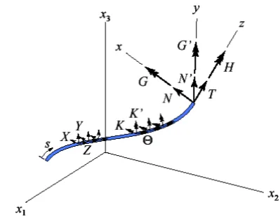
Figure 1 shows the strand geometry of a single layered helical strand , the developed geometry of the helix and also the forces such as normal, binormal , axial forces along the 3 directions perpendicular to each other and moments along the 3 directions perpendicular to each other. For the present problem, the core is assumed to be rigid radially.
[image:2.595.312.512.54.210.2]The equilibrium equations for the force and moment resultant have been derived for a general twisted and bent rod under the action of distributed forces and moments Figure 1 as a general case.
Fig. 1b. Forces and Moment distribution in a wire.
Sathikh et al [2] model made use of the concept of generalized strains derived by Ramsey (1988,1990) in the normal, binormal and tangential directions and adopted them as 1, 2, and 3 in place of the deformed curvature and twist used in the other models, after taking clue from Wempner [3].
Ramsey [4] & [5] has derived the following expressions for an axisymmetrical loading of a strand:
Wire flexural strain about the wire normal axis:
0
1
(2) Wire flexural strain about the wire binormal axis:r r ) sin 1 ( cos sin
cos2 2 2 2
2
(3)
Wire torsional strain about the wire axis:
r r
sin cos sin cos3 3
3
(4)
The binormal force ' '
1 G H
N equation is also
modified accordingly. The bending and twisting couples G' and H and the wire tension T was modified as mentioned:
1
EIG
(5) 2
J G
H (6) w
A E
T
(7) The resultant strand external force Fs and moment Ms can be obtained from the following equations, when the core deformations are also added.
c c s mT N E A
F [ sin
cos
](8) c c s J G r N Tr G H m M ] sin cos cos sin [
(9) EliminatingN
byG
andH
, and substitutingG
,H
and T in equations (8) and (9) would yield resultant external force and couple. Rearranging, the elements of stiffness matrix derived are presented below.
ni i i i i i i
[image:2.595.55.286.581.756.2]i i i i i i i C C I E J G r A E m A E F 1 2 2 2 4 3 ) sin cos ( sin cos sin (10)
n i i i i i i i i i i i i i i i i r I E J G r A E m M F 1 2 3 2 2 2 sin cos )] sin 1 ( sin [ cos sin (11) i i ni i i i i i i
i i i i i i c c I E J G r A E m J G
M
2
1 7 2 2
2 2 cos sin ) sin 1 ( sin cos sin
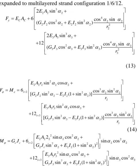
(12) Since the Sathikh model considered the curvature and twist effects with an appropriate contribution from the axial stress and has yielded the symmetry of stiffness matrix, as expected in any elastic system, it has been adopted as a basic theoretical model for this work.Stiffness coefficients of Sathikh et al model is expanded to multilayered strand configuration 1/6/12.
3 2 2 2
4
2 2 2 2
2 2 2 2 2 2 2
2 3
3 3 3
4
2 2 3 3
3 3 3 3 3 3 2
3
2 sin
6 cos sin
( cos sin )
2 sin
12 cos sin
( cos sin )
C C
E A
F E A
G J E I
r
E A
G J E I
r
(13)
2 2 2 2 2 2
3 2
2 2 2 2 2
2 2 2 2 2 2
2 2
3 3 3 3 3
3 2
3 2 2 3 3
3 3 3 3 3 3
3
sin cos
6 cos sin
[ sin (1 sin )]
sin cos
12 cos sin
[ sin (1 sin )] i
i
E A r
F M
G J E I
r
E A r
G J E I
r (14) 2 2
2 2 2 2 2 2
2 7 2 2 2 2
2 2 2 2 2
2 2
3 3 3 3 3 2
3 7 2 2 3 3
3 3 3 3 3 3
2 sin cos
6 sin cos
sin (1 sin ) sin cos
12 sin cos
sin (1 sin ) c c i
i
i
E A
M G J
G J E I
E A r
G J E I
(15)
The theoretical response of the strand under Fixed-Fixed loading and fixed free loading is estimated. In the case of Fixed-Fixed loading the ends is restrained from strand rotation. As the rotational strain () is zero they induce a torque in strand during axial loading.
In the case of free end, the ends of the strand are not restrained from angular displacement, and hence there is variation in strand rotation on strand axial load. Under Fixed-Free loading the strand moment Ms is considered as zero. The responses of the strand (axially loaded metallic cable made from 2 layers of wire helically wrapped around a central wire) is analytically determined for fixed & free boundary condition and compared with the test results of Utting and Jones [14].
III. EXTRACTION OF FINITE ELEMENT MODEL
A finite element model was developed to dimensions mentioned in the Table 1. The geometry of the core has been obtained by a linear z-axis extrusion. Each wire has been generated by the extrusion of its cross section along a
helix corresponding to the centroidal line of the wire. The simple straight strand cable structure has been constructed using the commercial CATIA software and was imported to ANSYS software for meshing & analysis. Three dimensional solid brick elements had been used for structural discretization. The model was developed for two pitch lengths for second layer for one pitch length for third layer and then meshed using 3D solid elements as shown in Figure 2 (a) to trade off between the computational time and accuracy.
The twisted elliptical cross sections of the wire normal to the core axis can be observed in Figure 2 (a). To consider the accuracy of results of the present finite element model, it was compared with experimental data reported by Utting [14]. In the experimental study the material modulus was determined to be 198000N/mm2. The diameters of the wire and core are 3.33 mm and 3.66 mm respectively with the wires laid up at a helix angle of 75.4°for first layer & 75.9°for second layer. An available ‘Master- Slave node concept’ called ‘CERIG’ (ANSYS command) was used to define a rigid region. Multiple constraint equations to relate nodes in the defined rigid region are automatically generated by this concept. In the present FE model, any plane cut perpendicular to the strand axis would contain nodes on the circular section of the core and those on the circular section of the wires.
Nodes on the rigid plane which is the loading end of the strand was grouped together to form ‘Slave nodes’. An additional node called ‘Master node’, which is the retained node for the rigid region was created on the axis of the core at a distance away from the slave nodes. This master node facilitates the axial loading. The nodes on the top surface of the wires and core (slave nodes) were automatically linked using rigid body elements to the master node to have the same displacement as defined by the master node. The Figure 1(b) is an illustration which shows the visibility of connection between the master node and the slave nodes with rigid links. High friction contact conditions were established between the wires and the core (wire/core contact), wire &wire have been applied for the nodes situated near the helical lines of contact between core and wires, wire &wire. Prediction of strand response for axial loading has been attempted for the fixed – fixed and free – fixed end conditions. Using these constraints the finite element analysis was performed to predict the forces acting on the strand.
TABLEI
GEOMETRICDATAOF 3LAYER19WIRESTRAND
Layer No. No. of wires Helical direction and angle Wire diameter Pitch length mm Young's modulus
N/ mm2
Poisson‘s ratio
1 1 - 3.66 mm - 198000 0.3
2 6 RH, 75.37o 3.33 mm 84.11 198000 0.3
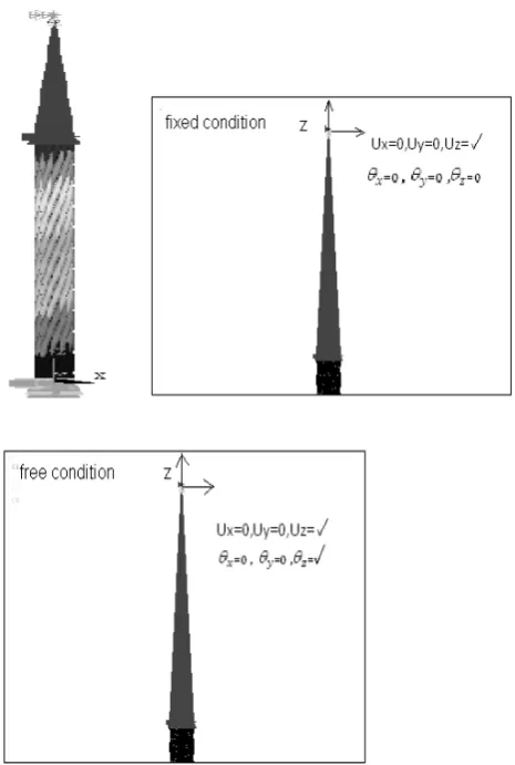
[image:3.595.55.291.50.150.2] [image:3.595.49.288.236.527.2]The boundary conditions required to simulate the loading for the strand model are mentioned as under:
The bottom end section of the cable is fully clamped by constraining all the d.o.f of the nodes are shown in Figure 3(a).
In the case of fixed end loading, strand rotation is clamped by constraining all the d.o.f of the master node except for its translational d.o.f along strand axis is shown in Figure 3(b).
Unlike the fixed end loading, in the case of free end loading, strand rotation about strand axis is permitted on the master node are shown in Figure 3(c).
IV. FINITE ELEMENT ANALYSIS RESULTS AND DISCUSSIONS
The responses of the strand assembly in terms of axial load, torque, contact parameters, and stress distribution to static axial displacement under two different degrees of fixity for a (1/6/12) steel strand have been studied using an finite element model. Emphasis is placed on the linear elastic global behavior of a simple isotropic straight steel strand under small strain. A linear kinematic hardening material model has been used. Rough frictional Contact between the center and helical wires, wire & wire contact have been simulated.
They can simulate general surface-to-surface contact with rough friction and sliding not permitted. Preliminary simulations performed with various finite element models of length up to many pitches, for trade-off between the computational time and accuracy justified the final selection of a 2 pitch in 2nd layer, 1 pitch in outer layer model (8x10⁴ nodes) used in this analysis. A strand axial strain of 0.01 at the master node was incremented in steps of 0.001 in the analysis and results have been compared with the Linear analytical extension model of Sathikh [2], and the experimental results of Utting & jones [14].
Figures 4 show the load response of the strand (at master node) to the axial strains for the fixed and the free end conditions.
In the case of fixed end loading, the linear limit of the strand force resulting from the present work is 71kN at an axial strain of 0.003. The corresponding strand force at the same strain from the theoretical model of expansion of Sathikh was observed to be 90kN. The experimental results of Utting & Jones (1988) were observed to be 71.5kN. The theoretical and the FEM findings resulted in a deviation of 20% and 0.7% respectively when compared with that of the test results.
In the case of free end loading, the linear limit of the strand force resulting from the present work is 29.5kN at an axial strain of 0.003. The corresponding strand force at the same strain from the theoretical model of extension of Sathikh was observed to be 32kN. The experimental results of Utting & Jones [14] were observed to be 28kN. The percentage of deviation of the theoretical and FEM findings with the test results was found to be 12.5%. and 5%
[image:4.595.47.287.66.211.2]Master node
Fig. 2a. Finite Element Mesh: (a) without master node (b) with master node (shown nearer to the top surface for clarity)
[image:4.595.308.549.396.543.2]
Figure 3. Finite Element Mesh: (a) bottom end fully clamped (b) fixed end loading condition (c) free end , loading condition.
[image:4.595.47.280.410.756.2]respectively. In general, it is confirmed that for the same strand axial strain, the helical wires with a free end condition carry less axial load than with the fixed end conditions. However, in the both the loading cases the finite element results tend to agree closely with that of the test results of Utting & Jones [14]. The very inclusion of Poisson’s effect in the formulation of stiffness matrix could narrow this deviation.
In the case of fixed end condition, as the ends are restrained from strand rotation, they induce torque which tends to untwist the strand during axial loading. Considering high friction also the play an vital role in increase of torque. Figure 5 shows the torque or moment variation.
In the case of free end, the ends of the strand are not restrained from angular displacement, and this variation in strand rotation is plotted as a Figure 6. The rotation values from the present case tend to agree with that of experimental values .
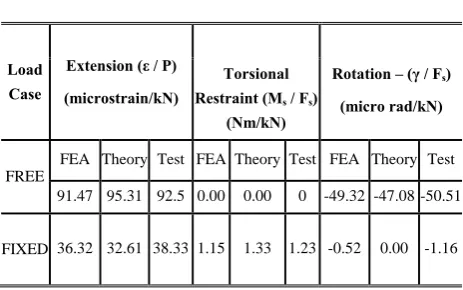
Table 2 shows the comparison of strand responses with the theory, present and test results.
The following are the observations of the finite element model:
(i) In the case of the fixed and free end loading, It is observed that for the same strand axial strain, the helical wires with a free end condition carry less axial load than with a fixed end. This is the reason that the axial (tensile) rigidity with the free end condition is less than that with a fixed end.
(ii) In the case of the fixed end loading, It is observed that for the same force, the helical wires with a fixed end condition torque is produced because of arresting the rotation. The percentage of deviation of the theoretical and FEM findings with the test results was found to be 20%. and 0.7% respectively
(iii)In the case of the free end loading, It is observed that for the same force the helical wires with a free end condition rotation is there because it is not restrained from angular displacement. The percentage of deviation of the theoretical and FEM findings with the test results was found to be 12.5% and 5% respectively. In general, the present of FEM model indicated a good correlation with the experimental findings.
(iv)For a constant strain value 0.05, stress distribution along Z axis for free end and fixed end condition are shown in Figure 7(a) and Figure 7(b) respectively. The Von Mises stress & maximum principal stress plots are also shown in Figure 7(c&e) and 7(d&f) for free end and fixed end condition respectively.
(v) In free end condition the maximum stress was found to be in concentrated in the core and its adjacent layer. In another words, the distribution of strand force is more in the core its adjacent layers. The percentage distribution of strand force between the wires in the layer is shown in Figure 8.
(vi)In the fixed end condition the ends of the strand are restrained from rotation and hence it tends to induce torque which again influences the stress levels in the outer layer. Also, the strand force was found to be more uniform between the layers and the core. This is again illustrated in Figure 8
[image:5.595.51.291.227.380.2](vii)These stress plots however represents the trend of stress distributions under axial loading which in turn would help the designer in finding the stress intensity locations. This would be very useful in design for strands.
[image:5.595.50.291.423.575.2]Fig. 5. Variation of torque with axial strain for fixed-end loading
Fig. 6. Strand rotational response for free end loading
TABLEII
COMPARISON OF STIFFNESS COEFFICIENTS WITH THEORETICAL,FEM
AND EXPERIMENTAL FINDINGS FOR BOTH END CONDITIONS
Load Case
Extension (ε / P)
(microstrain/kN)
Torsional Restraint (Ms / Fs)
(Nm/kN)
Rotation – (γ / Fs)
(micro rad/kN)
FREE
FEA Theory Test FEA Theory Test FEA Theory Test
91.47 95.31 92.5 0.00 0.00 0 -49.32 -47.08 -50.51
[image:5.595.47.279.641.786.2]V.CONCLUSION
In the present work, the global strand response were predicted using multilayer FE model and compared with extended equations of Sathikh [2] model cater to 3 layered wire rope strand and the published test results of Utting [14] for various end conditions, ranging from fixed end to free end. In general, the finite element results indicated a good correlation with the experimental values. Further, this model can provide information about the linear effects such as the stress distribution, their locations etc., which are otherwise difficult to address but do have an influence in the failure of the wire.
ACKNOWLEDGMENT
The authors are profoundly indebted to Professor Sathikh, S and Parthasarathy N.S for their constructive criticisms and extensive discussions during the period of this work.
REFERENCES
[1] A. Cardou and C. Jolicoeur C, “Mechanical Models of Helical Strands,” Applied Mechanics Review, vol. 50, no. 1, pp. 1-14, 1997. [2] S Sathikh., M.B.K. Moorthy and M. Krishnan, “A Symmetric Linear
Elastic Model for Helical Wire Strands under Axisymmetric Loads”,
Journal of Strain Analysis, Vol. 31, No. 5, pp. 389-399, 1996. [3] G Wempner. ‘Mechanics of solids with applications to thin bodies’,
McGraw-Hill, New York, 1973.
[4] H. Ramsey, “A theory of thin rods with application to helical constituent wires in cables”, International Journal of Mechanical Sciences, Vol. 30, No. 8, pp. 559-570, 1988.
[5] H .Ramsey. “Analysis of interwire friction in multilayer cables under uniform extension and twisting”, International Journal of Mechanical Sciences, Vol. 32 , No. 9, pp. 107-176, 1990.
[6] S.R. Ghoreishi., P. Cartroud., P. Davies and T Messager, “Analytical modeling of synthetic fiber ropes subjected to axial loads. Part I: A continuum model for multilayered fibrous structures”, International Journal of Solids and Structures, Vol. 44, No. 9, pp. 2924 – 2942, 2007.
[7] S.R. Ghoreishi., P. Cartroud., P. Davies and T Messager, “Analytical modeling of synthetic fiber ropes subjected to axial loads. Part II: A linear elastic model for 1+6 fibrous structures”, International Journal of Solids and Structures, Vol. 44, No. 9, pp. 2943-2960, 2007. [8] A. D. Carlson and R. G. Kasper, “A structural analysis of a
multiconductor cable,” Technical report, Naval underwater system center, New London laboratory, pp. 767 -963, 1973.
[9] W.G Jiang., M.S Yao. and J.M. Walton, “A concise finite element model for simple straight wire rope strand”, International Journal of Mechanical Sciences, Vol. 41, No. 2, pp. 143-161, 1999.
[10] W.G.Jiang, J.L Henshall. and J.M. Walton, “A concise finite element model for three-layered straight wire rope strand”, International Journal of Mechanical Sciences, Vol. 42, No. 1, pp. 63-89, 2000.
[11] S.R. Ghoreishi., P. Cartroud., P. Davies and T Messager, “Validity and limitations of linear analytical models for steel wire strands under axial loading, using a 3D FE model”, International Journal of Mechanical Sciences, Vol. 49, pp. 1251-1261, 2007.
[12] W.S. Utting and N. Jones, “The response of wire rope strands to axial tensile loads - Part I. Experimental results and theoretical predictions”, International Journal of Mechanical Sciences, Vol. 29, No. 9, pp. 605-619, 1987.
[13] W.S. Utting and N.Jones, “The response of wire rope strands to axial tensile loads - Part II. Comparison of experimental results and theoretical predictions”, International Journal of Mechanical Sciences; Vol. 29, No. 9, pp. 621-636. 1987.
[14] W.S. Utting and N. Jones, “Axial- Torsional interactions and wire deformation in 19-wire spiral strand” Journal of strain analysis, Vol. 23, No. 2 79-86, 1988.
[15] G. Shibu and N.S. Parthasarathy, “A concise mathematical approach for establishing a rotation restraint operating requirement for a bi-metallic strand cable”, International Journal of Theoretical and Applied Mechanics, Vol. 3, No. 3 pp.187-194, 2008.
Fig. 7. (a) stress distribution for free end condition along Z axis (b) stress distribution for fixed end condition along Z axis (c) Von-Mises stress for free end condition (d) Von-Mises stress distribution for fixed end condition (e) Max principle Stress for free end condition (f) Max principle Stress distribution for fixed end condition
[image:6.595.48.271.72.408.2] [image:6.595.58.209.628.745.2]