Abstract— Controlling robot vehicles has become one of the
most important applications in our automated world. Many control algorithms have been applied and used to accomplish the control task. Yet some of these robust algorithms still face stability and nonlinearity problems. In this paper we build a back propagation-based neural controller to do the control job. The said neural controller is trained according to the data collected from a controller that was pre-designed according to Lyapunov second theorem on stability. The neural controller is used to control a two-drive robot vehicle in such away to track a moving target in the plane and keep a fixed distance between the two. The trained neural controller is tested for shapes of target motion that were not seen during training.
Index Terms— Neural Controllers, Back Propagation Neural Networks, Robust Control Systems, Nonlinear Control Systems.
I. INTRODUCTION
Back propagation neural networks [1] [2] [3] are known for their ability to recognize patterns. The concept of pattern recognition could be further expanded beyond the idea of identifying faces and images. It could be expanded to cover other important fields in our life. Control applications are examples of these important fields [4]. In this paper we build a neural system capable of imitating another system in such a way that both of the systems will do approximately the same job in response to the same input. The original system we are talking about is a controller designed according to Lyapunov second method [5] [6] of stability and will be referred to as Lyapunov controller. The plant to be controlled is a robot vehicle that tries to track a moving target in the plane. The control action is divided into two sub-actions. The first is to control the vehicle speed in such away to keep a fixed distance between the vehicle and the moving target. The second is to govern the vehicle steering in order to keep the target tracking. These two actions could be thought of as independent or related actions. Consequently, we can have either one neural controller to control both steering and distance simultaneously, or we have two different controllers one for distance and the other for steering.
II. BACK PROPAGATION NEURAL NETWORKS
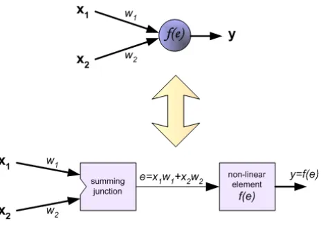
The basic structure of a back propagation neural network is shown in fig. 1. It simply consists of a group of mathematically identified modules called neurons shown in fig. 2. These neurons are distributed in layer forms and interconnected with each others via weights, which means
that each neuron receives a signal from the neurons in the previous layer, and each of those signals is multiplied by a separate weight value. The weighted inputs are summed, and passed through a limiting function which scales the output to a fixed range of values. The output of the limiter is then broadcast to all of the neurons in the next layer. So, to use the network to solve a problem, we apply the input values to the inputs of the first layer, allow the signals to propagate through the network, and read the output values.
Stimulation signal is applied to the input layer neurons and the response of the said layer propagates through the middle layers. Middle layers are referred to as hidden layers. Each connection between neurons has a unique weighting value. Fig. 2 shows the neuron structure. It simply receives input from the previous layer neurons. These inputs are weighted and summed to come up with a value to be applied to a nonlinear threshold function.
Back Propagation Neural Controller for a
Two-Drive Robot Vehicle
[image:1.612.316.540.304.400.2]Riyadh Kenaya, Member, IEEE, IAENG and Ka C Cheok, Member, IEEE
Fig. 1. General structure of a back propagation neural network.
[image:1.612.314.546.544.709.2]The said nonlinear function is usually an exponential function that ranges between two levels: 0 and +1 and the output value is passed on to the neurons in the next layer [7].
The connection weights in the neural network need to be tuned (adjusted) to obtain an overall response to certain stimulation in such a way to solve a particular problem. What makes each network different from another is the value of its weights. The process of adjusting the weights to come up with a response that is perfect or close to perfect is referred to as training. The training algorithm used in this paper is called back propagation (BP). It is an iterative process and based on collecting input/output data from a certain system we aim to imitate. The idea here is to adjust the weights to bring the response of the neural network close to the response of the original system, whenever the same stimulation is applied to the both.
At the beginning of the process of training, the weights are initialized to random values. The corresponding output is compared to the known-good output, and a mean-squared error signal is calculated. The error value is then propagated backwards through the network, and small changes are made to the weights in each layer. The weight changes are calculated to reduce the error signal for the case in question. The whole process is repeated for each of the example cases, then back to the first case again, and so on. The cycle is repeated until the overall error value drops below some pre-determined threshold. At this point we say that the network has learned the problem "well enough", yet the network will never exactly learn the ideal function, but rather it will asymptotically approach the ideal function. The mathematical derivation for the BP training algorithm is beyond the scope of this paper.
III. TWO WHEEL ROBOT VEHICLE
The block diagram of the robot vehicle to be controlled is shown in fig. 3. The said vehicle is equipped with a necessary set of sensors that provides the controller with the necessary information about the vehicle location (x and y coordinates) and the vehicle heading. It is also equipped with radar that gives information about the target location. This information is used to calculate both distance and heading error signals.
In1
In2 Out1
Out2
Subsystem Power am plifiers
Va Lef t
Va Right
Road inclinatn Lef t Speed Vl
Forward Vel Vf
Steer Vel Vs
Right Speed Vr
Subsystem Mobile Robot Motors & M otion
Vf
Vs X
Y
H
Subsystem M obile Robot
Kinem atics
Vr
Ul
Ur
Vl v olt l
Volt r
Subsystem L & R speed
controllers
Uf
Us Ul
Ur
Subsystem Forward & Steer
to Left & Right
conversion
0 Road Incli natn
The original controller is the above mentioned Lyapunov controller. The design details of the said controller are beyond the scope of this paper.
The data used to train the BP neural network are all collected from Lyapunov controller. The error signal vector and control signal vector are both the input/output data to be used in training process.
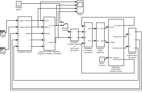
Fig. 4 shows the overall system that contains the robot vehicle as a plant and Lyapunov controller as a plant governor.
Y target X target
X target
Y target
X
Y
H Dis t Error
Hdg Error
Heading
X
Y
Subsystem sensors
In1
In2 Out1
Out2
Subsystem power ampl ifi ers
Va Lef t
Va Right
Road inclinatn Lef t s peed Vl
F orward Vel Vf
St eering Vel Vs
Right s peed Vr
Subsystem mobile robot motors & motion
Vf
Vs X
Y
H
Subsystem mobile robot
kinematics Uf
Us Ul
Ur
Subsystem forward & steeri ng
to left & right conversion
Vr
Ul
Ur
Vl Volt l
Volt r
Subsystem L & R speed
controll ers Scope
0
Road incli natn Manual
swi tch Ds t Err
Hdg Err
Heading
X
Y Ds t Ctrl
Hdg Ctrl
Lyapunov MRAC subsystem di stance & heading controllers 0
Constant speed
The target is simulated by a cross in the plane. It takes its motion from two independent signal generators for x and y axes.
Fig. 5 shows the Lyapunov controlled vehicle tracking the moving target.
IV. LYAPUNOV CONTROLLER DATA
[image:2.612.312.544.175.326.2]Fig. 6 shows Lyapunov controller and sensor block diagrams. Both the distance and steering error signals are applied to the controller. The controller generates two output control signals, one for distance control and the other for steering control. It is important to mention that the design of Lyapunov controller is based on a second order reference model [8]. The main purpose of Lyapunov controller here is to build a control system that generates control signals in the same way a linear second order reference system generates. Accordingly, the cost function we try to minimize is the error difference between the second order controller and its
Fig. 3. Robot vehicle block diagram.
Fig. 4. Lyapunov controller for the robot vehicle.
[image:2.612.71.295.542.726.2]corresponding Lyapunov one. As a result, this method makes the nonlinear system behave like a linear system whose control parameters (like overshoot and steady state error) are design values to be set by the designer.
Ytarget Xtarget
Xtarget
Y target
X
Y
H
Dist Error
Hdg Error
Heading
X
Y
Subsystem Sensors
Dst Err
Hdg Err
Heading
X
Y Dst Ctrl
Hdg Ctrl
Lyapunov Controller
Figs. 7-10 show Lyapunov controller data. These data are collected in response to a sinusoidal target motion in the plane. In this experiment we desire to make the vehicle track the target and keep three feet of distance between the two.
Figs. 11 and 12 show the overall vehicle response to the target motion. One can easily tell that Lyapunov controller just does the right control job. One can also see that the distance between the two is almost kept constants and close to 3 feet.
V. MIXED SIGNAL-BASED NEURAL CONTROLLER RESULTS
The data given in figs. 7-12 are used as training data for the BP neural controller. Distance and heading error signals are considered as stimulation data, and the corresponding distance and steering control signals are considered as response data. In this section, both of the distance and heading error signals would be treated as members of one stimulation vector. The said vector is refereed to as error vector. In the same sense, the distance and steering control signals are considered as members of the same response vector and referred to as control vector.
The network structure is shown in fig. 13. It is a two layer network and this is one of many possible structures. In our design, we choose 15 TANSIG neurons for the first layer and one PURLIN neuron for the second layer. The first layer weight matrix is W115X2. W22X15 is the second layer matrix.
s1 y1 s2 y2
1 Out1
y2 tansi g
purel i n netsum1 netsum
W2* u
Matri x Gai n Wei ght W2 W1* u
Matrix Gain Weight W1
b2* u
Matrix Gain Bi as B2 b1* u
Matrix Ga in Bi as B1
1 Constant
1 1
Consta nt 1 In 1
u
W1 matrix dimensions give indication to the number of neurons and input variables applied to the network. 15 is the number of neurons, whereas 2 is the number of variables applied. B115X1 is the bias matrix for the first layer.
Fig. 6. Robot vehicle Lyapunov controller
Fig. 7. Lyapunov controller distance error signal.
Fig. 8. Lyapunov controller distance control signal.
Fig. 9. Lyapunov controller heading error signal.
[image:3.612.90.280.110.227.2]Fig. 10.Lyapunov controller heading control signal.
[image:3.612.314.542.126.187.2]Fig. 11. Robot vehicle tracking the moving target (x-axis tracking).
Fig. 12. Robot vehicle tracking the moving target (y-axis tracking).
B21X1 is the second layer bias. The training epoch number
is chosen to be 50. Increasing the epoch number may result in reducing the training mean square error.
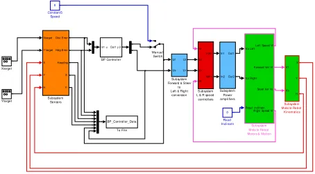
The trained network replaces the original Lyapunov controller and the experiment is rerun. Fig. 14 shows the overall control system with the BP neural network as the system controller. Notice how the distance error and heading error signals are combined in one vector. Also, the control signals for distance and heading are both combined in one control vector.
Ytarget Xtarget
BP_Control l er_Data
To Fi l e Xtarget
Y target
X
Y
H Dist Error
Hdg Error
H eading
X
Y
Subsystem Sensors
In1
In2 Out1
Out2
Subsystem Power ampl i fi ers
Va Lef t
Va R ight
R oad inclinatn Lef t Speed Vl
F orward Vel Vf
Steer Vel Vs
R ight Speed Vr
Subsystem M obi le Robot Motors & Motion
Vf
Vs X
Y
H
Subsystem M obi l e Robot
Ki nem ati cs
Vr
U l
U r
Vl v olt l
Volt r
Subsystem L & R speed control l ers Uf
Us U l
U r
Subsystem Forward & Steer
to Left & Right conversion
0 Road Incl i natn
Manual Swi tch
0 Constant5
Speed
In1 uOut1 y 2
BP Controll er
Figs. 15-20 show the neural system performance when exposed to the same operational conditions that the original controller has witnessed.
0 50 100 150 200
-10 0 10
Time (s)
T
a
rg
e
t
m
o
ti
o
n
a
n
d
v
e
h
ic
le
t
ra
c
k
s
ig
n
a
ls x-target motion
x-vehicle motion
0 50 100 150 200
-5 0 5
Time (s)
T
a
rg
e
t
m
o
ti
o
n
a
n
d
v
e
h
ic
le
t
ra
c
k
s
ig
n
a
ls y-target motion
y-vehicle motion
VI. SEPARATE SIGNAL-BASED NEURAL CONTROLLER
RESULTS
In this section, we break the neural controller introduced in the previous section into two different controllers. One for distance, and the other, for heading control. Each one of these two controllers is trained independently from the other. This gives us some flexibility in choosing different training parameters for the two controllers. The importance of this measure is represented by the ability of selecting certain range of training data for one controller and selecting another range for the other. Even the epoch number and number of neurons per layer of one of the controllers could be completely different from those of the other. We have trained the distance controller based on the data collected from the original controller while tracking the target that moves in a sinusoidal shape. On the other hand, the heading controller is trained based on the data collected from the original controller while tracking the target whose motion is of step shape. The reason we went with two different types of training data, is to ensure the maximum stability of the neural controller. Our experiments have shown that choosing any other set of training data did always cause an unstable behavior of the robot vehicle.
Figs. 21-26 show the performance of the separate signal controller. One can easily notice that the three systems (Lyapunov, separate, and mixed signal controllers) have almost the same response to the same excitation. It is obvious that the three systems show stable behavior for a sinusoidal target motion. The three controllers succeed in keeping a fixed distance of 3 feet between the vehicle and the target.
Fig. 14. Back propagation neural controller for the robot vehicle.
[image:4.612.314.541.50.126.2]Fig. 16. BP neural controller distance control signal.
Fig. 17. BP neural controller heading error signal.
Fig. 18.BP neural controller heading control signal.
Fig. 19.BP neural controller overall tracking signals (x-axis motion).
Fig. 20.BP neural controller overall tracking signals (y-axis motion).
[image:4.612.72.299.186.312.2]0 50 100 150 200 -10 0 10 Time (s) T a rg e t m o ti o n a n d v e h ic le t ra c k s ig n a
ls x-Target motion
x-vehicle motion
0 50 100 150 200
-5 0 5 Time (s) T a rg e t m o ti o n a n d v e h ic le t ra c k s ig n a
ls y-target motion
y-vehicle motion
VII. GENERALITY OF BPNEURAL CONTROLLERS
Generality of any neural system is represented by its ability to respond to the excitations that were not seen during
training [6] [9]. In this section we test the BP mixed signal controller for special types of target motion. A mixture of step and sinusoidal Target motion is an example of these excitations that were not seen during training. The neural controller behavior is compared with that of Lyapunov controller (Figs. 27 and 28). It is obvious that Lyapunov controller shows a very poor performance. It completely diverges away from the target after few seconds of relative stability. On the other hand, we can see that the mixed signal neural controller retains its stability and tries to reduce the sudden error caused by the target step motion (figs. 29 and 30). This error reduction is affected by the robot vehicle moment of inertia.
0 50 100 150 200
-100 0 100 Time (s) T a rg e t m o ti o n a n d v e h ic le t ra c k s ig n a ls x-target motion x-vehicle motion
0 50 100 150 200
-100 0 100 Time (s) T a rg e t m o tio n a n d v e h ic le t ra c k s ig n a ls y-Target motion y-Vehicle motion
0 50 100 150 200
-10 0 10 Time (s) T a rg e t m o ti o n a n d v e h ic le t ra c k s ig n a ls x-Target motion x-Vehicle motion
0 50 100 150 200
-10 0 10 Time (s) T a rg e t m o ti o n a n d v e h ic le t ra c k s ig n a
ls y-Target motion
y-Vehicle motion
VIII. CONCLUSIONS AND FUTURE WORK
Lyapunov controllers could be substituted with back propagation neural controllers. The neural controllers show stable behavior and accurate tracking. Mixed signal
Fig. 21. Separate signal BP neural controller distance error signal.
Fig. 22. Separate signal BP neural controller distance control signal.
Fig. 23. Separate signal BP neural controller heading error signal.
Fig. 24. Separate signal BP neural controller heading control signal.
Fig. 25. Separate signal BP neural controller x-axis tracking signals.
Fig. 26. Separate signal BP neural controller y-axis tracking signals.
Fig. 27.Lyapunov controller overall tracking signals (x-axis target step
motion).
Fig. 28.Lyapunov controller overall tracking signals (y-axis target sinusoidal
motion).
Fig. 29.BP mixed signal neural controller overall tracking signals (x-axis
target step motion).
Fig. 30.BP mixed signal neural controller overall tracking signals (y-axis
controllers could be also replaced with their separate signal counterparts. Signal separation enables us to use different sets of training parameters for the independent controllers. It also makes it easy for us to use different sets and combinations of training vectors. We still get the system to work and perform well.
The future work would highly concentrate on optimizing the length of training data chains and studying the effect of selecting certain parts of data other than using the whole data chain. This is to be done by eliminating the redundant parts of data and retain the part that conveys core and non-repetitive information. This would result in reducing the training time and the hardware size needed to realize the network. Neural network optimization is considered as one of the most challenging research topics.
REFERENCES
[1] J. –S. R. Jang, C. T. Sun, and E. Mizutani, Neuro Fuzzy and Soft
Computing. Prentice Hall, 1997.
[2] Z. Effendi, R. Ramli and J.A. Ghani, “Back Propagation Neural
Networks for Grading Jatropha curcas Fruits Maturity,” American
Journal of Applied Sciences, 7 (3): 390-394, 2010.
[3] Michael C.O'Neill, “Training back-propagation neural networks to define
and detect DNA-binding sites,” Nucleic Acids Research, Vol. 19, No. 2,
313.
[4] Panos J. Antsaklis, “Neural Networks in Control Systems,” IEEE
Control Systems Magazine,” April 1990.
[5] M. Kanat Camlibel, Jong-Shi Pang, and Jinglai Shen, “Lyapunov
Stability of Complementarily and Extended Systems,” 2006 Society for
Industrial and Applied Mathematics, Vol. 17, No. 4, pp. 1056-1101.
[6] R. Kenaya, Euclidean Adaptive Resonance Theory with Application to
Nonlinear and Adaptive Control Systems, PhD Dissertation, Oakland University, Rochester, Michigan, 2009.
[7] T. Catfolis, “Mapping a Complex Temporal Problem into a Combination
of Static and Dynamic Neural Networks,”SIGART Bulletin, Vol. 5, No.
3.
[8] P. Vempaty, K. Cheok, and R. Loh, “Model Reference Adaptive Control
for Actuators of a Biped Robot Locomotion,” Proceedings of the World
Congress on Engineering and Computer Science, Vol. II ,WCECS October 20-22, 2009, San Francisco, USA.
[9] C. Cox, K. Mathia, J. Edwards, and R. Akita, “Modern Adaptive Control
With Neural Networks,” International Conference on Neural Networks
Information Processing, ICONIP 96, Hong Kong.