Abstract—Internet users rely on the good capabilities of
TCP/IP networks for dealing with congestion. The network delay and the number of users change constantly, which might lead to transmission problems. Usually, they are handled following approaches such as drop tail or random early detection (RED) algorithms. During the last few years, automatic control techniques are providing practical solutions. Moreover, if there are wireless links, congestion control is more difficult to detect. This paper presents a methodology to design a PID controller with a linear gain scheduling that allows a network with wireless links to deal with control congestion under a variety of configurations. The proposed technique is demonstrated through non-linear simulations and compared with the classical PID
Index Terms— PID, Westwood TCP/AQM, congestion
control, robustness, gain scheduling.
I. INTRODUCTION
HE importance of Internet cannot be denied. However, there are situations in which problems arise such as long delays in delivery, lost and dropped packets, oscillations or synchronization problems ([1], [2]). Congestion is responsible for many of these problems. It is harder to detect if there are wireless links in the network. Thus, techniques to reduce congestion are of great interest. There are two basic approaches ([3], [4]): congestion control,
which is used after the network is overloaded, and
congestion avoidance, which takes action before the
problem appears.
Feedback control can help to solve congestion control. The end-to-end transmission control protocol (TCP), and the active queue management (AQM) scheme define the two parts implemented at the routers’ transport layer where congestion control is carried out. The most common AQM objectives ([5]) are: efficient queue utilization (to minimize
the occurrences of queue overflow and underflow, thus reducing packet loss and maximizing link utilization),
queuing delay (to minimize the time required for a data
packet to be serviced by the routing queue) and robustness
(to maintain closed-loop performance in spite of changing conditions).
Manuscript received April 2012. This work was supported in part by AECI under project AP/039213/11 and by MiCInn project DPI2010-21589-C05-05.
T. Alvarez is with the University of Valladolid (Tlef: +34 983423162; e-mail: [email protected]).
In general, AQM schemes enhance the performance of TCP, although they have some disadvantages as they do not work perfectly in every traffic situation. Numerous algorithms have been proposed (a good survey can be found in [4]). The most widely used AQM mathematical models were published in [5]. Since then, several control approaches have been published: fuzzy, predictive control, robust control, etc. The automatic control technique that has received more attention is the PI controller, followed by the PID ([6]).
AQM techniques should be robust and give good results when the network is not operating in nominal situation, when the delays are changing, or the number of users or the intensity of the packets’ flow vary, i.e. the network should deliver the users’ data on time and without errors regardless of the changes in the working parameters.
So, the AQM congestion control algorithm should be robust, stable and perform in a changing environment. If PID is chosen as the AQM algorithm, there are many useful references in the literature: [7] and [8] cover quite a lot of the situations that can arise. Reference [9] gives a graphical characterization of the stable region of a PID controller applied to the AQM router, but they do not consider changing traffic conditions. These works are of special interest because they explicitly consider delays in the design of the PIDs and this is the situation that arises when working with networks: a system with delay.
Motivated by these issues, this paper presents how to derive PIDs with guaranteed stability and robustness that performs well under a network with wireless links and changing traffic conditions. The work presented in this paper applies the generic method by [7] for finding stable PID controllers for time delay systems in the dynamic TCP Westwood/AQM router model. A linear gain scheduling is included in the design (reducing the gain variation) to enhance the robustness and ensure adequate behaviour in extreme working scenarios. The metrics applied to study the controller performance are: the router queue size (real value and standard deviation), the link utilization and the probability of packet losses.
Non-linear simulations will show the fine performance of the technique by applying it to a problem of two routers connected in a Dumbbell topology, which represents a single bottleneck scenario. The length of their queues is controlled with a PID whose properties are guaranteed following the results presented in the paper.
This paper is organized as follows. Section 2 briefly describes TCP Westwood. A fluid flow model is presented in Section 3 and, in Section 4, the methodology is described. Simulation results are shown in section 5. Finally, some
Design of PID Controllers for TCP/AQM
Wireless Networks
Teresa Alvarez
conclusions and discussion on future work are presented. II. TCP WESTWOOD
TCP Westwood (TCPW) ([10]-[14]) is a modification of TCP NewReno at the source side, intended for networks where losses are not only due to congestion such as the wireless networks studied in this paper. The protocol from the receiver point of view is the same in both TCPs, but there are some changes in the way the source calculates the available bandwidth. These modifications affect the dynamics of the system, which justifies the necessity of specific controllers for TCPW.
In TCPW, the congestion window increases during the slow start phase, but is the same as in NewReno during the congestion avoidance phase. A packet loss is indicated by a coarse timeout ending or the reception of three Duplicate ACKnowledgeS (DUPACKS). The basic idea of TCPW is to use the flow of returning ACKs to estimate the available bandwidth (BWE); then this value is used for setting the size of the slow start threshold size (sstresh) and the
congestion window (cwnd) ([10]):
IF (3 DUPACKS are received) THEN sstresh = (BWE*RTTmin)/MSS IF (sstresh<2) THEN sstresh=2 cwnd = sstresh;
IF (coarse timeout expires) THEN sstresh = (BWE*RTTmin)/MSS IF (sstresh<2) THEN sstresh=2 cwnd = 1;
IF ACKs are successfully received THEN
cwnd is increased following the RFC2581 document for congestion control
This TCPW captures the basic NewReno behavior, but Westwood improves the stability of the TCP multiplicative decrease.
III. FLUID FLOW MODEL FOR TCP WESTWOOD This section presents a fluid flow model derived in [10]. As in the original approach ([5]), there is a single bottleneck. Now all the TCP connections are assumed to follow the Westwood formulation.
A. Nonlinear Model
The nonlinear model used for the simulations is described by the following two coupled nonlinear differential equations:
0
2 0 0 0 0 0 1 R t p T C R t q R t W T R t p T C R t q R t W t W T C t q W p p p p (1)
0 , 0 max 0 t q if C t W T C t q N t q if t W T C t q N C q p p (2)
Where
W: average TCP window size (packets),
q: average queue length (packets),
R: round-trip time = q/C+Tp (secs), C:link capacity (packets/sec), Tp: propagation delay (secs),
NTCP=N: load factor (number of Westwood TCP
sessions) and
p: probability of packet mark.
Equation 1 describes the TCP window control dynamic and Equation 2 models the bottleneck queue length as an accumulated difference between the packet arrival rate and the link capacity. The queue length and window size are positive, bounded quantities, i.e., q
0,q andW
0,W ,where q and W denote buffer capacity and maximum
window size, respectively.
B. Linearized Model
Although an AQM router is a non-linear system, a linearized model is used to analyze certain required properties and design controllers. To linearize (1) and (2), it is assumed that the number of active TCP sessions and the link capacity are constant, i.e., NTCP(t)=NTCP=N and C(t)=C.
As described in [5] and [10], the dependence of the time delay argument t−R on the queue length q is ignored and it
is assumed to be fixed to t−R0. This is a big assumption and
there could be situations where it would not be acceptable. In [15], it was deduced that this is a good approximation when the round-trip time is dominated by the propagation delay. When the model is linearized, the same supposition is made. It cannot be denied that the calculations are significantly simplified, but further research in the matter would be advisable.
Then, local linearization of (1) and (2) around the operating point
q0,p0,W0
results in the followingequations:
) ( 1 ) ( ) ( 1 2 1 2 1 0 0 0 0 2 2 0 0 0 2 0 0 0 0 0 0 t q R t W R N t q R t p R T N C R T T R R t q t q C R R T R t W t W C T R N t W p q p p q (3)where Tq0 R0Tp and W(t)WW0 and
0
p p p
(W,q) as the state and p as input, the operating point
q0,p0,W0
is defined by W 0 and q0, that is,
00 3 2 0 0 0 2 0 p T R N T R R W W p p , 0 0
0 q N W
q . (4)
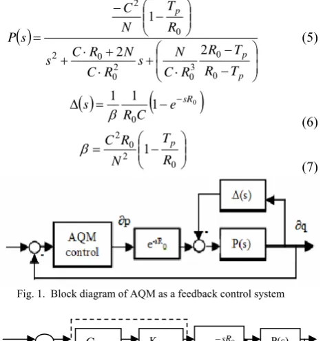
Equation (3) can be further simplified by separating the low frequency (‘nominal’) behavior P(s) of the window dynamic from the high frequency behavior ∆(s), which is considered parasitic. Taking (4) as the starting point and following steps similar to those in [5], we can obtain the feedback control system (Fig. 1) for TCPW/AQM ([16]).
The action implemented by an AQM control law is to mark packets with a discard probability p(t) as a function of
the measured queue length q(t). Thus, the larger the queue,
the greater the discard probability becomes.
p p p T R T R R C N s R C N R C s R T N C s P 0 0 3 0 2 0 0 2 0 2 2 2 1 (5)
1 1
1 0
0
sR
e C R
s
(6)
[image:3.595.59.294.268.516.2] 0 20 2 1 R T N R C p (7)
Fig. 1. Block diagram of AQM as a feedback control system
Fig. 2. Block diagram of the AQM feedback control system
IV. CONTROLLER DESCRIPTION
This section presents the approach that has been followed to deal with the AQM congestion control problem in a network with wireless links under varying traffic.
Some parameters, such as the link capacity C, do not
usually change, but the round trip delay R0 and the number
of users NTCP vary frequently. The proposed technique is
simple, but works well in networks with a wide range of users and varying delays.
As network traffic changes constantly, this affects the performance of the system. We tune the PID for a certain set of conditions, but they change. The method proposed here will improve the router’s performance no matter how many users or how much delay there is in the network.
The PID is tuned following a model-based approach, taking the linearized dynamic model of TCPW described in
previous section as the starting point. Fig. 2 depicts the block diagram corresponding to the feedback control approach followed in the paper: P(s) is the transfer function obtained in Section 3. The delay esR0is explicitly
considered in the design. There are two elements in the controller C(s):
1.CPID(s) is a PID controller and
2.K1 is a variable gain; a simple gain scheduling that allows
the controller to work satisfactorily in a broad range of situations.
The steps in the design are:
1.Choose the worst network scenario in terms of NTCP and
R0: i.e., the biggest delay and the smallest number of
users.
2.Choose the best network scenario in terms of NTCP and R0:
i.e., the smallest delay and the biggest number of users. 3.Design a controller CPID(s) that is stable in these two
situations and the scenarios in between.
4.Add a simple gain scheduling K1 to improve the system’s
response, based on the expected variations of the system’s gain.
We have chosen the PID controller (Equation 8, [6]) as the AQM congestion control algorithm, as it is the most common form of feedback control technique and relevant results can be found in the literature regarding the stability properties and the tuning. The structure of the controller is:
t d i p t d i p dt t de K d e K t e K dt t de T d e T t e K t u 0 0 1 (8)The PID should be tuned to be stable in the above mentioned situations. It is also required to have good responses in terms of settling time and overshoot. Thus, the tuning of the controller is done following the method presented in [7]: the system can be of any order and the roots can be real or complex. Using the provided Matlab toolbox, a three dimensional region is obtained. Kp, Ki and
Kd chosen inside this region give a stable closed-loop
response.
The simple gain scheduling approach proposed in the paper takes into consideration the big gain variation that the AQM dynamic model has:
0 2 1 R T N C p (9)
Moreover, if a fair comparison among all the network configurations were done, the open-loop gain of the systems should be the same, so the independent term of the denominator of the transfer function should be included:
p p T R T R R C N 0 0 3 0 2 (10)
This term greatly affects the size of the stable region and the magnitude of the PID’s tuning parameters (as will be shown in next section). So we take out this term from P(s) and calculate the stable region for:
1 1 ) ( 2 s a s s P sPnormalized n (11)
And:
s P Ps P T R
T R N
R C
s P T R
T R R C
N
R T N C s P
n cte
n p p
n
p p p
0 2 0 2
2 0 3
0 0 3 0
0 2
2 2
1 )
(
(12)
So, the gain scheduling term is given by (13).
20 3
2
2 0
0 1
2
R C
N T R
T R K
p p
(13)
It is important to choose the worst and best scenarios properly. A good knowledge of the network is required.
In the next section the network parameters are defined. The stable regions are depicted and the PID is tuned. Then, linear and non-linear simulations will show the goodness of the method.
V. SIMULATIONS
A. Tuning the controller
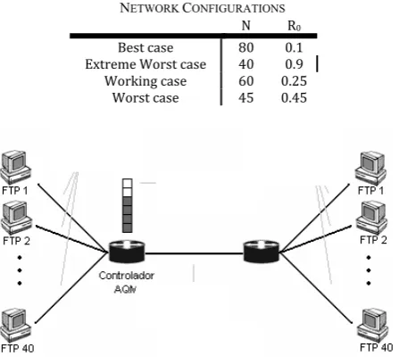
The basic network topology used as an example to test the controller is depicted in Fig. 3. It is a typical single bottleneck topology. The link capacity (C) is kept constant
in all experiments. Although this parameter could change, its adjustments are more related with network updates than with everyday traffic conditions. The different scenarios come from changing the number of users (N) and the round
trip time (R0) (see Table 1).
TABLEI
NETWORK CONFIGURATIONS
N R0
Best case 80 0.1
Extreme Worst case 40 0.9 Working case 60 0.25
Worst case 45 0.45
Fig. 3. Dumbbell topology
[image:4.595.55.294.56.238.2]The situations deal with a broad range of conditions: few users and big delay, many users and small delay and in-between situations. As can be seen, the worst situation (extreme worst case) is when the number of users is 40 and the round trip delay is 0.9 seconds. The best situation has a delay of only 0.1 seconds and 80 users.
Fig. 4 shows the open loop poles of the system for the best and extreme working scenarios, without considering the delay. The lower graphs depict the open loop poles and zeros if a Padé approximation of first order is used. The other scenarios have their poles and zeros between these two situations.
best
Real Axis
Im
agi
na
ry
A
x
is
-1 -0.5 0
-1 -0.5 0 0.5 1
extreme
Real Axis
Im
agi
na
ry
A
x
is
-20 -10 0 10 20
-4 -2 0 2 4
best w ith delay
Real Axis
Im
agi
na
ry
A
x
is
-4 -2 0 2 4
-1 -0.5 0 0.5 1
extreme w ith delay
Real Axis
Im
agi
na
ry
A
x
is
-8 -6 -4 -2 0
[image:4.595.308.545.123.328.2]-4 -2 0 2 4
Fig. 4. Open loop poles and zeros
The open loop step response for each of the studied scenarios of the original linear system (P(s)) and the
normalized one (Pn(s)) are shown in Fig. 5 (upper and
lower, respectively). The step has amplitude of 0.01 because the input of the system is the probability of marking a packet and it always takes values between 0 and 1. In fact, the smaller the changes, the better for the system.
Both systems have the same settling time, but as will be shown later in the section, the behavior once the loop is closed will be very different. The worst scenario gives the slowest open loop response (settling time: 14.7 seconds) and the best scenario gives the fastest one (settling time: 0.74 seconds).
0 5 10 15 20 25 30
1000 -500 0 500
P(s): open loop step responses w ith delay
Time (sec)
0 5 10 15 20 25 30
-5 0 5 10 15x 10
-3 Pn(s): open loop step responses w ithout delay
Time (sec)
A
m
pl
itude best
w orking w orst
[image:4.595.60.284.478.682.2]w orstextreme
Fig. 5. Step responses
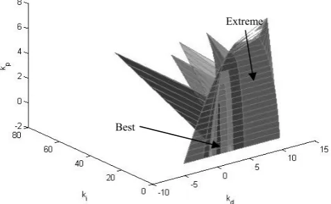
Let us consider the normalized transfer function approach. Using Hobenbichler’s approach ([7]), the 3-dimensional stable region for the PID is depicted in Fig. 6. The color code is the same as in Fig. 5. Note that if Kp, Ki
and Kd are chosen inside these regions, the closed loop
[image:4.595.305.547.502.711.2]is stable in all the working scenarios: the best, the worst and those in between. Maybe the controller is not the best for each of the cases, but it would work well in all of the scenarios.
[image:5.595.310.545.129.323.2]Moreover, due to the normalization in the transfer function, the scales of the graph are in the same range or magnitude, making the tuning of the controller easier.
Fig. 6. Stable region with proposed method
This is clearer if we see the same 3-dimensional representation for the system without the methodology proposed in the paper. In Fig. 7, the stable regions are shown, but the scales are in the range of 10-3 to 10-4.
Moreover, the PID controller will give a worse performance, as will be shown in the simulations. It is more difficult to see where all the regions overlap.
In [17] and [18], the effect of N and R0 on the size of the
controller’s stability region was studied. They concluded (and our experiments also agree with their result) that the smallest stability region is obtained for the smallest number of users (N) and the minimum round trip delay (R0) ( Fig. 7
shows the region).
Fig. 7. Stable region with classical approach
B. Linear Simulations
The controller’s parameters, when the method proposed in the paper is applied, are chosen as Kp=0.5, ki=0.3
kd=0.01. Fig. 8 shows the closed loop step response of the
linear systems for the four scenarios under study. The settling time is small and all the systems have a settling time smaller than 15 seconds.
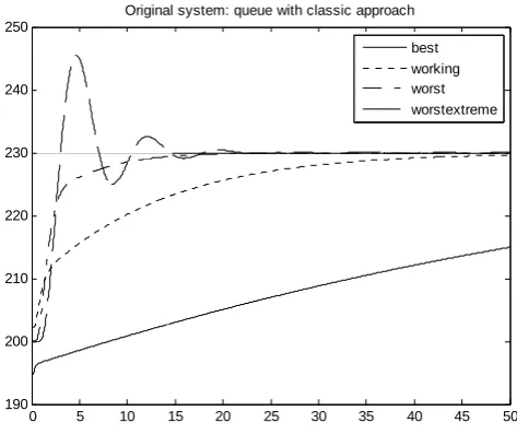
If the classical approach is followed, the controller parameters are Kp= -4·10-5, ki= -10-5 and kd= -2·10-5. As
shown in Fig. 9, the settling times are very different. The best case scenario has a settling time around 250 seconds and the worst extreme is much faster (10 seconds). These settling times are very different: there are two orders of magnitude between them. This way, it is not feasible to have the same PID controller giving good closed-loop responses.
0 5 10 15 20 25 30 35 40 45 50
-0.2 0 0.2 0.4 0.6 0.8 1 1.2 1.4
Closed loop step response w ith proposed approach
[image:5.595.49.288.149.296.2]Time (sec) best w orking w orst w orstextreme
Fig. 8. Closed-loop step response with proposed method As can be seen, using the approach presented in the paper (Fig. 8), the settling times have the same order of magnitude and the same PID can work well for all the scenarios.
0 50 100 150 200 250 300 350 400 450 500
-0.2 0 0.2 0.4 0.6 0.8 1 1.2 1.4
Closed loop step response w ith classic approach
Time (sec) best
w orking w orst w orstextreme
Fig. 9. Closed-loop step response with classical approach
C. Nonlinear Simulations
Taking the model described in Section III and the controllers described in Section IV, the following experiments were carried out.
In the first experiment, the reference is set to 230 packets (30 above the working point). Looking at the probability of marking a packet, there are not many differences between the two approaches (Figs. 10 and 11). However, the graphs with the queue evolution (Figs. 12 and 13) show significant differences. It should be noted that the settling time when the proposed method (Fig. 12) is applied is smaller than when the classic approach is followed (Fig. 13). As was expected, the slowest response corresponds to the system with the biggest number of users.
Best
Extreme
Best
[image:5.595.310.544.388.579.2] [image:5.595.49.288.487.644.2]0 5 10 15 20 25 30 35 40 45 50 0
0.01 0.02 0.03 0.04 0.05 0.06 0.07 0.08
Original system: probability with new approach
[image:6.595.51.281.52.242.2]best working worst worstextreme
Fig. 10. Experiment 1, probability with new method
0 5 10 15 20 25 30 35 40 45 50 0
0.01 0.02 0.03 0.04 0.05 0.06 0.07 0.08
Original system: probability with classic approach
[image:6.595.317.551.53.248.2]best working worst worstextreme
Fig. 11. Experiment 1, probability with classic approach
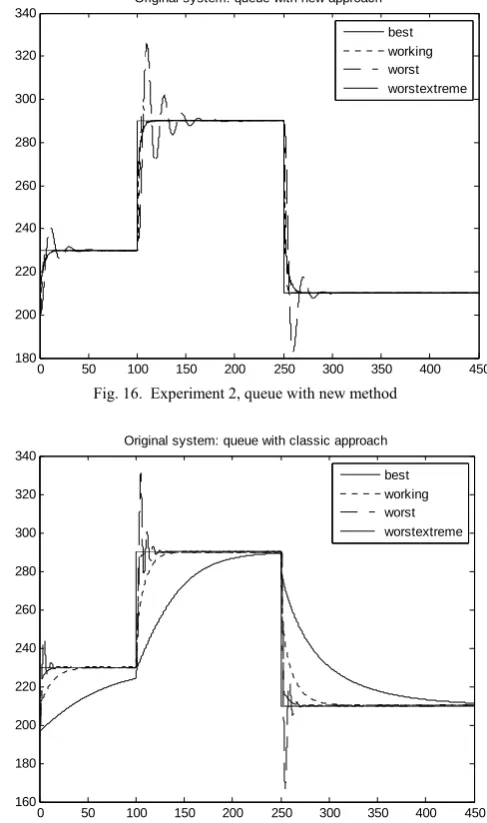
In experiment 2, a variable reference was applied. First, the queue set-point (in packets) was increased by 30, then by 60 and finally decreased by 80 packets. All the plants performed well (Fig. 14-17).
The performance of the system follows the same patterns as in experiment 1. Fig. 14 shows the evolution of the probability for the proposed method. The peaks are smaller than when using the classic approach (Fig. 15).
Fig. 16 shows the queue values with the modified PID. Clearly, the settling times are smaller than when the classic approach (Fig. 17) is followed (as happened in the first experiment).
Again, the slowest response corresponds to the system with the biggest number of users
0 5 10 15 20 25 30 35 40 45 50 195
200 205 210 215 220 225 230 235 240 245
Original system: queue with new approach best working worst worstextreme
Fig. 12. Experiment 1, queue with new method
0 5 10 15 20 25 30 35 40 45 50 190
200 210 220 230 240 250
[image:6.595.306.543.281.485.2]Original system: queue with classic approach best working worst worstextreme
Fig. 13. Experiment 1, queue with classic approach
Finally, let us consider an experiment where the number of users (N) changes dynamically.
The network default configuration is the working scenario described in Table I. The set point does not change and is equal to the queue nominal value (200 packets).
The changes in the number of users are depicted in Fig. 18 and the probability and queue size for the classic and proposed approaches in Fig. 19 and Fig. 20, respectively.
Looking at Fig. 19, we can conclude that the changes and the real value of the probability are smaller with the new method. Smaller probability values mean that the probability of discarding packets is smaller.
[image:6.595.51.285.284.481.2]0 50 100 150 200 250 300 350 400 450 0
0.02 0.04 0.06 0.08 0.1 0.12 0.14
[image:7.595.57.294.55.254.2]Original system: probability with new approach best working worst worstextreme
Fig. 14. Experiment 2, probability with new method
0 50 100 150 200 250 300 350 400 450 0
0.02 0.04 0.06 0.08 0.1 0.12 0.14 0.16 0.18 0.2
Original system: probability with classic approach best working worst worstextreme
Fig. 15. Experiment 2, probability with classic method The mean, standard deviation and variance for the queue size following the classic and the new approach are shown in Table II. The reference is set to 200 packets and the mean value for the proposed methodology is 201.4 packets. This is a value very close to the reference, especially if we compared it with the mean of 210 packets of the classic approach.
TABLEII
MEAN AND VARIANCE RESULTS
Mean St. dev Var
Classic 210.5 37.3 1393.4
New 201.4 31.9 1019.7
0 50 100 150 200 250 300 350 400 450 180
200 220 240 260 280 300 320 340
[image:7.595.309.553.56.468.2]Original system: queue with new approach best working worst worstextreme
Fig. 16. Experiment 2, queue with new method
0 50 100 150 200 250 300 350 400 450 160
180 200 220 240 260 280 300 320 340
[image:7.595.61.296.273.472.2]Original system: queue with classic approach best working worst worstextreme
Fig. 17. Experiment 2, queue with new method
VI.CONCLUSION
The paper has presented a PID design with linear gain scheduling and normalized values that works very well under different network traffic conditions. The controller is tuned for the worst scenario and works properly in a wide range of situations.
As we are working with TCP Westwood, the analysis of the results is valid either in wired or wireless routers. Linear and nonlinear simulations confirm the technique’s potential. This is especially convenient, as many design procedures are tested in restricted situations with no guarantee that the controller will behave similarly in other scenarios.
The technique presented in the paper gives more uniform results than the classical approach. It does not matter if the scenario is close to the nominal situation or a worst case setting, the controller reacts adequately and the settling times are all of the same order. The classic approach cannot deal well with extreme situations.
50 60 70 80 90 100 110 120 130 140 150 45
50 55 60 65 70 75 80
N: Number of users
Fig. 18. Changing N
0 10 20 30 40 50 60 70 80 90 100 0.01
0.015 0.02 0.025 0.03 0.035
Probability
classic new
Fig. 19. Probability when the number of users changes
0 10 20 30 40 50 60 70 80 90 100 50
100 150 200 250 300 350
Queue
[image:8.595.47.285.47.696.2]classic new
Fig. 20. Queue size when the number of users changes
ACKNOWLEDGMENT
The author would like to thank Prof. F. Tadeo for so many fruitful discussions.
REFERENCES
[1] Azuma, T., T. Fujita, M. Fujita (2006). Congestion control for TCP/AQM networks using State Predictive Control. Electrical Engineering in Japan, 156, 1491-1496.
[2] Deng, X., S. Yi, G. Kesidis. C.R. Das (2003). A control theoretic approach for designing adaptive AQM schemes. GLOBECOM’03, 5, 2947 – 2951.
[3] Jacobson, V. (1988). Congestion avoidance and control. ACM SIGCOMM’88.
[4] Ryu, S., C. Rump, C. Qiao (2004). Advances in Active Queue Management (AQM) based TCP congestion control. Telecommunication Systems, 25, 317-351.
[5] Hollot, C.V., V. Misra, D. Towsley, W. Gong (2002). Analysis and Design of Controllers for AQM Routers Supporting TCP flows. IEEE Transactions on Automatic Control, 47, 945-959.
[6] Aström K.J. and T. Hägglund (2006), Advanced PID control. ISA. NC.
[7] Hohenbichler, N. (2009). All stabilizing PID controllers for time delay systems. Automatica, 45, 2678-2684.
[8] Silva, G., A. Datta and S. Bhattacharyya. PID controllers for time-delay systems. Birkhäuser, 2005.
[9] Long, G.E., B. Fang, J.S. Sun and Z.Q. Wang (2010). Novel Graphical Approach to Analyze the Stability of TCP/AQM Networks. Acta Automatica Sinica, 36, 314-321.
[10] M. di Bernardo, L. A. Grieco, S. Manfredi, and S. Mascolo," Design of robust AQM controllers for improved TCP Westwood congestion control", Proceedings of the 16th International Symposium on Mathematical Theory of Networks and Systems (MTNS 2004), Katholieke Universiteit Leuven, Belgium, July, 2004.
[11] Chen, J., F. Paganini, M.Y. Sanadidi, R. Wang and M. Gerla (2006). Fluid-flow analysis of TCP Westwood with RED. Computer Networks, 50, 132-1326.
[12] Mascolo, S., C. Casetti, M. Gerla, M.Y. Sanadidi, R. Wang. TCP Westwood: bandwidth estimation for enhanced transport over wireless links, in: Proceedings of Mobicom, 2001.
[13] Wang, R., M. Valla, M.Y. Sanadidi, B. Ng, M. Gerla, Efficiency/friendliness tradeoffs in TCP Westwood, in:IEEE Symposium on Computers and Communications, Taormina, Italy, July 2002.
[14] Wang, R., M. Valla, M.Y. Sanadidi, M. Gerla, Adaptive bandwidth share estimation in TCP Westwood, in: Proceedings of IEE Globecom, Taipei, 2002.
[15] Hollot, C.V. and Y. Chait (2001). Nonlinear stability analysis for a class of TCP/AQM networks”. In Proceedings of the 40th IEEE Conference on Decision and Control, Orlando, USA.
[16] Alvarez, T. (2012). Designing and Analysing Controllers for AQM routers working with TCP Westwood protocol. (Internal Report, University of Valladolid. To be submitted).
[17] Al-Hammouri, A.T. , V. Liberatore, M.S. Branicky, and S.M. Phillips (2006b). Parameterizing PI congestion controllers. Proc. First International Workshop on Feedback Control Implementation and Design in Computing Systems and Networks, Vancouver, CANADA. [18] Al-Hammouri, A.T., V. Liberatore, M.S. Branicky, and S.M. Phillips