Digital soil mapping from conventional field soil observations

Digital Soil Mapping from Conventional

Field Soil Observations

Juraj BALKOVIČ

_{, Zuzana RAMPAŠEKOVÁ}

_{, Vladimír HUTÁR}

_,

Jaroslava SOBOCKÁ

_{and Rastislav SKALSKÝ}

1_{International Institute for Applied Systems Analysis, Laxenburg, Austria;} 2_Department

of Soil Science, Faculty of Natural Sciences, Comenius University in Bratislava, Slovak Republic; 3_{Department of Geography and Regional Development, Faculty of Natural Sciences,}

Constantine the Philosopher University in Nitra, Slovak Republic; 4_{Soil Science}

and Conservation Research Institute, Bratislava, Slovak Republic

Abstract

Balkovič J., Rampašeková Z., Hutár V., Sobocká J., Skalský R. (2013): Digital soil mapping from conven-tional field soil observations. Soil & Water Res., 8: 13–25.

We tested the performance of a formalized digital soil mapping (DSM) approach comprising fuzzy k-means (FKM) classification and regression-kriging to produce soil type maps from a fine-scale soil observation network in Rišňovce, Slovakia. We examine whether the soil profile descriptions collected merely by field methods fit into the statistical DSM tools and if they provide pedologically meaningful results for an erosion-affected area. Soil texture, colour, carbonates, stoniness and genetic qualifiers were estimated for a total of 111 soil profiles using conventional field methods. The data were digitized along semi-quantitative scales in 10-cm depth intervals to express the relative differences, and afterwards classified by the FKM method into four classes A–D: (i) Luvic Phaeozems (Anthric), (ii) Haplic Phaeozems (Anthric, Calcaric, Pachic), (iii) Calcic Cutanic Luvisols, and (iv) Haplic Regosols (Calcaric). To parameterize regression-kriging, membership values (MVs) to the above A–D class centroids were regressed against PCA-transformed terrain variables using the multiple linear regression method (MLR). MLR yielded significant relationships with R2 _{ranging from 23% to 47% (P < 0.001) for classes A, B and D, but only marginally significant for}

Luvisols of class C (R2 _{= 14%, P < 0.05). Given the results, Luvisols were then mapped by ordinary kriging and the} rest by regression-kriging. A “leave-one-out” cross-validation was calculated for the output maps yielding R2 _{of 33%,} 56%, 22% and 42% for Luvic Phaeozems, Haplic Phaeozems, Luvisols and also Regosols, respectively (all P < 0.001). Additionally, the pixel-mixture visualization technique was used to draw a synthetic digital soil map. We conclude that the DSM model represents a fully formalized alternative to classical soil mapping at very fine scales, even when soil profile descriptions were collected merely by field estimation methods. Additionally to conventional soil maps it allows to address the diffuse character in soil cover, both in taxonomic and geographical interpretations.

Keywords: field soil description; fuzzy k-means; pedometrics; regression-kriging; terrain

Digital soil mapping (DSM) has become popular for producing maps of soil classes and properties from spatially explicit soil inventories and from

al. 1997). DSM integrates many statistical and geo-information tools and concepts, including supervised and unsupervised classifications (De Gruijter & McBratney 1988; Burrough et al. 1997; Carré & Girard 2002; Hengl et al. 2004b; Lagacherie 2005; Zádorová et al. 2011), geostatistics (Webster & Oliver 2007), environ-mental correlations and scorpan-based models (McKenzie & Ryan 1999; McBratney et al. 2003). A thorough review of DSM methods and their applications in soil science was published by McBratney et al. (2003).

The DSM techniques can represent a formal-ized alternative to the conventional soil mapping, where both the soil classification and mapping are handled numerically. The soil profiles are classified in terms of taxonomic distance or membership to centroids of soil classes, enabling more soil variables to be addressed simultaneously (Mc-Bratney & De Gruijter 1992; Zhu et al. 2001; Carré & Girard 2002). The fuzzy k-means method (FKM, Bezdek et al. 1984) has recently become especially popular for classification purposes as it enables to represent a continuous character and uncertainty in mapped soils. Once classified, the soil profile partitions are then interpolated into membership maps, which are used instead of conventional soil maps. Increased availability of remote sensing and GIS data has promoted the regression-kriging method (Odeh et al. 1994, 1995) as a generic interpolation tool for the map-ping purposes (Hengl et al. 2004b). That is the reason why we chose regression-kriging and FKM as major components in our DSM model. Some authors emphasize co-kriging as a superior method for mapping undersampled soil properties when auxiliary covariates are available (Kalivas et al. 2002; Penížek & Borůvka 2006). However, this method is more cumbersome and yields only a small benefit when soil and auxiliary variables are weakly correlated (Ahmed & De Marsily 1987).

Soil profile surveys have always been the basic strategy for soil type mapping regardless of whether or not the maps were produced with the use of DSM. Although a lot of attention has been paid to coupling of DSM with various soil information systems (McBratney et al. 2003), only few ap-plications used soil profile descriptions gathered solely by empirical field observation methods (e.g. Carré & Girard 2002). This approach in-volves several implications compared to measured analytical data. Firstly, the horizon properties

are usually described using various qualitative or semi-quantitative scales (e.g. Schoeneberger et al. 2002), where the continuous soil variables are ranked along discrete empirical categories. This ranking may negatively affect numerical classifica-tion if the attribute space is not correctly designed. Secondly, the resultant numerical partition may not be fuzzy enough to provide meaningful soil-terrain relationships.

In this article we add to the above context by testing the performance of a simple DSM approach to produce soil type maps from a network of com-mon field profile descriptions from the study area in Rišňovce, Slovakia. We also examine whether the standard morphological descriptions compris-ing the qualitative and semi-quantitative horizon properties collected in the field fit adequately into the statistical DSM tools. Additionally, we evaluate if this approach provides pedologically meaning-ful outputs for very fine scales in erosion-affected landscape – both in taxonomical and geographical interpretations.

MATERIAL AND METHODS

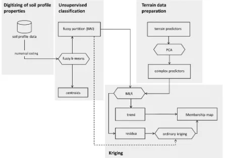
Model description. The presented DSM model

(Figure 1) integrates (i) digitizing of soil profile properties, (ii) unsupervised FKM classification of soil profiles, (iii) auxiliary terrain data prepara-tion, and (iv) kriging of soil membership maps.

As concluded by Burrough et al. (1997) and De Gruijter et al. (1997), the FKM classification can produce meaningful soil typological results. It partitions soil profiles into the given k classes, where profile properties in the class centre are represented by centroids. The centroid membership values MV(m_ij) follow the criteria given by Eq. (1):

(1)

where:

n – total number of profiles

k – number of classes

Several authors have suggested hybrid interpola-tions combining kriging and linear regression with terrain variables as powerful methods for mapping soil classes when soil distribution was closely cor-related with terrain (e.g. Odeh et al. 1994, 1995; Goovaerts 1999; Hengl et al. 2004a). Among the hybrid interpolation techniques, regression-kriging (Odeh et al. 1994, 1995) was identified

 



_

_



ij m i n m j k

as the most superior method by Knotters et al. (1995) and Bourennane et al. (2000). It couples Multiple Linear Regression (MLR) with kriging, as given by Eq. (2):

(2)

where:

mˆ_j(s₀) – MV of class j at a non-sampled location s₀ q_l(s₀) – l-th predictor at location s₀

β_l – parameter of predictor l in MLR

p – number of predictors used for soil class j

ε_j(s_i) – MLR residual at a sampled location s_i w_i – weight of the kriging operator

The weights, w_i, depend on the distances between the observations and the predicted location s₀ and spatial relationships between sampled data around the predicted location. While geographic distances are here determined by X and Y coordi-nates as Euclidean distance, spatial relationships are described by the experimental semivariogram from values of Eq. (3) as stated in Burgess & Webster (1980):

₍₃₎

where:

γˆ(h) – semivariance

h – separation lag-distance between locations

s_i and s_i+h

ε(s_i), ε(s_i+h) – MLR residuals at locations s_iand s_i+h d(h) – number of pairs at any separation distance h

The semivariogram is a quantitative measure of how the semivariance between the sampled points is reduced as separation distance decreases, and it can be modelled by some of the authorised semivariogram equations (cf. Webster & Oli-ver 2007). The weighting factors of Eq. (2) are estimated by solving the kriging equations (Bur-gess & Webster 1980). Regression-kriging is a powerful method when the correlation between soil and terrain variables is high and the MLR residuals are spatially correlated (cf. Hengl et al. 2004a). When MVs do not yield any signifi-cant linear relationship with terrain predictors, the regression-kriging interpolation can then be

Figure 1.Scheme of the digital soil mapping algorithm, including the fuzzy k-mean classification of soil profiles, PCA transformation of terrain predictors and regression-kriging of soil membership maps





 p

l

n

i i j i l

j s q s w s s

mˆ( 0) ₁ 1 ( 0) ₁ ( 0) ( )









 d

i si si h

h d

h _{1 ( ) ( )}2

) ( 2

replaced by ordinary kriging by omitting the MLR component from Eq. (2).

The transformation of terrain predictors by Prin-cipal Component Analysis (PCA) was suggested by Hengl et al. (2004a) to reduce multicollinearity in MLR. Therefore the Principal Components (PCs) are here considered as complex terrain variables which are uncorrelated and standardised and can therefore be used instead of the original terrain predictors (e.g. Gobin et al. 2001; Hengl et al. 2004a).

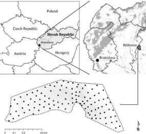
Study area and soil sampling. The study area

covers approximately 37 ha of arable land in the cadastral area of Rišňovce in Slovakia (Figure 2). The soils here are mainly Haplic Phaeozems (An-thric, Calcaric), Luvic Phaeozems (Anthric), Calcic, Cutanic Luvisols and Haplic Regosols (Calcaric), which are significantly affected by erosion.

The soil cover was studied using a grid sampling layout composed of parallel downslope transects, trying to ensure that all soil elements are repre-sented in the grid (Figure 2). The between-sample distances in transects were slightly shorter than distances between transects: the inter-sample distance was 70 m on average. A total of 111 soil profiles were sampled using the hand auger equip-ment. This study was performed by the same re-searchers to minimize the inter-observer variability. The following profile properties were estimated using the field handbook by Schoeneberger et

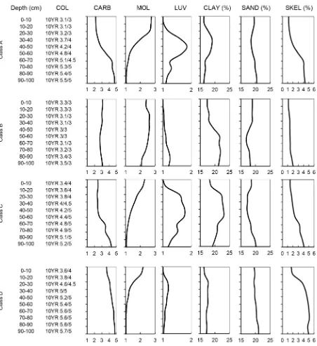
al. (2002): (i) horizon nomenclature, comprising master horizons and other modifiers, and horizon thickness (in cm), (ii) soil matrix colour in the moist state using the Munsell notation, (iii ) tex-ture class by the field hand test, (iv) carbonates by the effervescence field test, and (v) stoniness in vol. %. All genetic horizons were sampled up to a maximum of 100 cm depth.

Digitizing of soil profile properties. The soil

horizon data were digitized using the following rules: (i) Munsell colours were converted into the CIELab coordinates (COLX, COLY, and COLZ) using the method published by Melville and Atkinson (1985), (ii) soil texture estimates were converted into central sand and clay contents (SAND, CLAY in %) of the respective texture classes of the USDA triangle, (iii) carbonate esti-mates (CARB) were placed along a 1 to 5 ordinal scale; the numbers stand for non-effervescent, very slightly effervescent, slightly effervescent, strongly effervescent, and violently effervescent soils, (iv) stoniness remained in the percentage (SKEL), and (v) soil horizons were rated by the intensity of illuvial silica clay accumulation (LUV) and mollic properties (MOL), which are two main processes in the studied soils, using the following ordinals: 1 – not applicable; here the layer does not constitute a part of either A or B horizon, 2 – weak; here the layer constitutes a part of A or

B horizon, but the horizon does not meet all the criteria for mollic Am or luvic Bt horizon, and 3 – intense; here the layer constitutes a part of the Am or Bt horizon. The above variables were digitized by 10-cm depth intervals to gather the vertical profile stratification. The soil variables were distinguished by a depth interval and a prop-erty name: e.g. 10_SAND stands for sand content in the 0–10 cm layer. As a result, 89 variables were constructed for each soil profile (luvic properties were omitted for the topmost soil layers). The above digitizing avoids too many zero values in the input data, which could cause deviations in the FKM classification.

Auxiliary terrain variables. The digital

eleva-tion model (DEM) was constructed in 5-m resolu-tion from detailed altimetry measurements using the RBF technique in Geostatistical Analyst for ArcGIS software (Johnston et al. 2001). The altimetry data were measured by Leica ATX900 GG GNSS receiver with real-time correction for sub-cm precise positioning provided by the Slovak Space Observing Service. The DEM resolution reflects both positional accuracy and density of measurements. The following terrain variables were calculated from DEM: (i) slope steepness in degrees (SLP), (ii) planar and profile curva-ture (PLANCURV, PROFCURV; cf. Moore et al. 1991), (iii) overland flow accumulation in metres calculated from filled DEM (FLW, 3 × 3 kernel, cf. Maidment 2002), and (iv) topographic wet-ness index (TWI, cf. Wilson & Gallant 2000). Detailed information concerning the above terrain variables is presented in Table 1.

PCA was calculated for the terrain variables in STATISTICA software (StatSoft Inc. 2003), thus aiming to reduce collinearity and to extract com-posite terrain gradients as mapping predictors. FLW and SLP variables were log-transformed prior to PCA. Hereafter, the PCA factor coordinates of

cases for PC1–6 were considered as DSM predic-tors (cf. Hengl et al. 2004a).

Fuzzy k-means classification. The FKM

classifi-cation was calculated in FuzME software (Minasny & McBratney 2002) using diagonal distance, number of classes k = 4, and fuzziness coefficient φ = 1.5. The fuzziness coefficient was optimized as suggested by McBratney and Moore (1985). The number of classes respects the number of soil typological units recognised in the study area during the soil survey. Centroids were interpreted according to WRB nomenclature (FAO-ISRIC-ISSS 2006).

In addition, PCA and Detrended Correspondence Analysis (DCA) were calculated for soil profile data in STATISTICA and CANOCO (ter Braak & Šmilauer 2002) software to explore inner vari-ability in the profile data matrix.

Kriging interpolation. The fuzzy MVs were

interpolated using the regression-kriging Eq. (2). However, ordinary kriging (Burgess & Web-ster 1980) was used when no significant linear relationships were observed between MVs and terrain predictors. Parameterization of regression-kriging included (i) MLR analysis between MVs and PC1–6 terrain predictors at sampled loca-tions independently for each soil centroid; where βcoefficients and ε residuals were calculated, and (ii) semivariance analysis and semivariogram model estimation with the ε residuals. We used 5 × 5 neighbourhood averaging for PC1-6 ras-ters in order to obtain “balanced” predictor val-ues at the sampled locations, and a conventional semivariogram analysis was performed with MVs when ordinary kriging was used. Kriging weighting factors for both ordinary and regression kriging were estimated by solving the kriging equations. All the analyses were calculated in R programme (www.R-project.org) using the following choices: Ordinary Least Squares (OLS) for MLR and

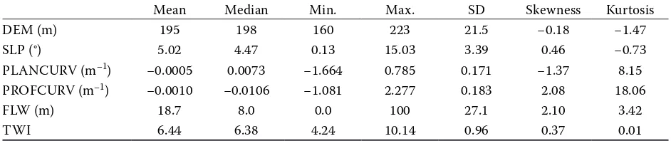
punc-Table 1.Descriptive statistics of terrain variables

Mean Median Min. Max. SD Skewness Kurtosis

DEM (m) 195 198 160 223 21.5 −0.18 −1.47

SLP (°) 5.02 4.47 0.13 15.03 3.39 0.46 −0.73

PLANCURV (m–1_{) −0.0005 0.0073 −1.664 0.785 0.171 −1.37 8.15}

PROFCURV (m–1_{) −0.0010 −0.0106 −1.081 2.277 0.183 2.08 18.06}

FLW (m) 18.7 8.0 0.0 100 27.1 2.10 3.42

TWI 6.44 6.38 4.24 10.14 0.96 0.37 0.01

tual technique for kriging. The exponential model of Eq. (4) was used to calculate the semivariogram (Webster & Oliver 2007):

(4)

where:

c₀ – error (nugget) variance

c₁ – so-called “partial sill” variance

r – “lag” distance

The DSM algorithms were run over PC1-6 terrain predictors independently for each soil type to render the membership maps with 5m cell resolution. Given the averaging-to-the-mean effects of interpolation, the assumption of composite variables given by Eq. (1) was violated in the output MV maps. This error was corrected by the equalizing variance trans-formation with respect to the original MV matrix, and each voxel of the transformed MV rasters was afterwards rescaled so that the sum of its MVs was equal to one.

A cross-validation “leave-one-out” approach was used to validate the DSM model. It uses a loop function over observation data leaving a profile out of the mapping analysis when a prediction is calculated for that particular profile. Pearson’s cor-relation coefficients (r) and the linear regression model with R2 _{and F-test P values were used to test} the significance of such predictions.

We used the pixel-mixture technique (De Gruijter et al. 1997) to visualize the soil type distribution using the algorithm published for R programme at http://spatial-analyst.net/wiki/ index.php?title=Uncertainty_visualization.

RESULTS AND DISCUSSION

Fuzzy k-means classification

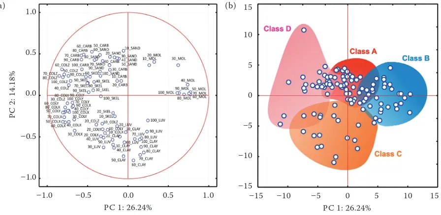
The ordinations of soil profiles (n = 111) and their properties (m = 89) in attribute space were analysed using PCA (Figure 3). An attribute space of linear ordinations is appropriately configured when profile attributes are linearly related to principal components. We examined this assumption by DCA as introduced by ter Braak and Šmilauer (2002), who suggested the maximum length of gradient expressed in SD of the attribute turnover along the ordination axis to be a measure of data heterogeneity. Given this measure, an input data matrix is suitable for linear ordinations when the DCA gradient length is less than 4 SD. The value of 0.95 SD in our analysis indicates that the input matrix is properly shaped for both PCA and FKM analyses. Additionally, we do not expect any severe deviations in PCA and FKM calculations caused by too many zero values in the input matrix since this was avoided with data digitizing.





)

(h c0c1   h r



Figure 3. Principal Component Analysis (PCA) scatter plot of the soil profile data projected at the first two prin-cipal components (40.4% of the total eigenvalue): (a) factor coordinates of attributes, and (b) factor coordinates of profiles; shaded areas outline where the fuzzy k-means (FKM) class maxima are plotted; PCA analysis was based on correlation; notation of soil variables: “Depth_property”

(a)

PC 1: 26.24% PC 1: 26.24%

PC

2

: 1

4.

18%

–1.0 –0.5 0.0 0.5 1.0 –15 –10 –5 0 5 10 15 1.0

0.5

0.0

–0.5

–1.0

15

10

5

0

–5

–10

–15

Following the resultant ordination in the PC1-2 quadrate (Figure 3) we judge that semi-quantitative and ordinal profile data demonstrate quite a con-tinuous ordination pattern which conditions proper FKM classification. Shaded areas in Figure 3b outline profiles which have their MV maxima in the particular FKM classes. It is quite clear that

profiles with their MV maxima in class A consti-tute the most homogeneous sample, whereas the other classes, and especially classes C and D, are internally more heterogeneous.

The FKM analysis yields four class centroids (A–D), which were interpreted as Luvic Phaeo-zems (Anthric), Haplic PhaeoPhaeo-zems (Anthric,

caric, Pachic), Calcic Cutanic Luvisols, and Haplic Regosols (Calcaric), respectively. Additional infor-mation needed to support the classification was provided by the Soil Science and Conservation Research Institute in Bratislava, Slovakia, from auxiliary data sources. Vertical distributions of the studied profile properties in particular centroids are illustrated in Figure 4. Whereas class A and C centroids represent more or less climax soils, the class B centroid depicts colluvic soils with topsoil material accumulated via tillage-induced erosion, and the class D centroid comprises strongly eroded soils with only shallow remnants of mollic and luvic horizons. Apparently, the soil erosion and accumulation are fundamental forces affecting the taxonomical variety of soils in this study area. The MVs contain a significant portion of fuzzi-ness and the overall confusion index (Burrough et al. 1997) averaged 0.62. When aggregated by class maxima, the average confusion index values were 0.66, 0.47, 0.79 and 0.62 for A to D classes, respectively.

The highest confusion was calculated for Luvisols, which represent a minority soil type in the study area since only 14 out of 111 soil profiles were clas-sified as Luvisols during the field survey. In contrast, Phaeozems of class B are clearly determined by its centroid as they show the lowest confusion index.

Composite terrain gradients

To a certain extent, the terrain gradients were collinear since they were all derived from DEM. In particular, DEM yields significant Pearson’s correlations with FLW, PROFCURV, SLP and TWI (r = –0.08, –0.30, –0.11 and –0.07, respectively, all P < 0.01). The overland flow accumulation (FLW) significantly correlates with all the other variables: r = –0.32, 0.18, 0.28 and 0.30 for PLANCURV, PROFCURV, SLP and TWI, respectively. Finally, PLANCURV significantly correlates with PROF-CURV (r = –0.28) and TWI (r = –0.41), and TWI

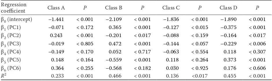
Table 3.Results of multiple linear regression method (MLR) between PC1-6 terrain predictors and log-transfor-med MVs of classes A to D

Regression

coefficient Class A P Class B P Class C P Class D P

β₀ (intercept) –1.441 < 0.001 –2.109 < 0.001 –1.836 < 0.001 –1.890 < 0.001 β₁ (PC1) –0.071 < 0.172 0.365 < 0.001 –0.127 < 0.015 –0.375 < 0.001 β₂ (PC2) 0.243 < 0.001 –0.201 < 0.017 –0.088 < 0.159 –0.164 < 0.017 β₃ (PC3) –0.019 < 0.805 0.472 < 0.001 –0.144 < 0.057 –0.229 < 0.006 β₄ (PC4) –0.149 < 0.170 0.052 < 0.717 –0.063 < 0.554 0.118 < 0.307 β₅ (PC5) 0.148 < 0.164 –0.559 < 0.001 0.118 < 0.264 0.373 < 0.001 β₆ (PC6) 0.364 < 0.255 –0.568 < 0.182 0.030 < 0.925 0.176 < 0.606

R2 _{0.233 < 0.001 0.466 < 0.001 0.136 <0.017 0.455 < 0.001}

β₀–β₆ – MLR coefficients; P – probability for F-test values; R2 _{– coefficient of determination of MLR}

Table 2. Principal Component Analysis (PCA) outputs; correlation coefficients between PC1–6 and the original terrain variables

Transf. PC1 PC2 PC3 PC4 PC5 PC6

DEM (m) no –0.22 0.41 –0.75 –0.34 0.32 –0.03

FLW (m) log 0.50 –0.53 –0.42 0.45 0.27 0.12

PLANCURV (m–1_{) no –0.69 0.19 0.36 0.36 0.47 –0.07}

PROFCURV (m–1_{) no 0.56 –0.34 0.43 –0.47 0.40 0.00}

SLP (°) log –0.38 –0.87 –0.20 –0.06 –0.06 –0.22

TWI no 0.85 0.41 –0.03 0.22 0.02 –0.24

Eigenvalue 1.960 1.523 1.095 0.724 0.568 0.131

yields significant correlations with PROFCURV at r = 0.23 and SLP at r = –0.63.

Because of the established collinearity, PCA was used to calculate new, uncorrelated terrain vari-ables. The factor coordinates for PC1 to 6, which are linear combinations of the original terrain variables (Table 2), are considered new composite and uncorrelated terrain variables inputting the DSM model. A contribution of PC1-6 to the total PCA matrix eigenvalue is also shown in Table 2.

Kriging of membership maps

The β coefficients and residuals ε of MLR be-tween log-transformed MVs and PC1-6 predictors

of Eq. (2) were calculated using the OLS method. All the MLR models were statistically significant at P < 0.05 (Table 3), however, the explained variance strongly varied with soil classes: R2 _{was between} 14% and 47%. Haplic Phaeozems of class B and Haplic Regosols of class D, which are essentially affected by erosion and accumulation processes, respond to terrain variables better than the others (R2_{= 0.47 and 0.46 for class B and D,} respective-ly). In contrast, Cutanic Luvisols of class C show only a weak, although still significant response (R2 _{= 0.14). The spatial distribution of Luvisols is} explained rather by local outcrops of clay sediments than by terrain forces in the study area.

The class A–D residuals ε had almost normal distributions, although they were not all perfectly

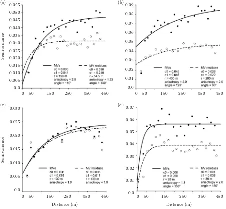
Figure 5. Exponential semivariogram models of MV (solid line) and their residuals (dashed line): (a) class A – Lu-vic Phaeozems, (b) class B – Haplic Phaeozems, (c) class C – Cutanic Luvisols, and (d) class D – Haplic Regosols

Distance (m)

Se

m

iv

ar

ia

nc

e

Se

m

iv

ar

ia

nc

e

Distance (m) 0 50 150 250 350 450

0.055 0.050 0.045 0.040 0.035 0.030 0.025 0.020 0.015 0.010 0.005 0.0

0 50 150 250 350 450 0 50 150 250 350 450 0 50 150 250 350 450

0.030

0.025

0.020

0.015

0.010

0.005

0.0

0.09 0.08 0.07 0.06 0.05 0.04 0.03 0.02 0.01 0.0

0.07

0.06

0.05

0.04

0.03

0.02

0.01

0.0

(a) (b)

Gaussian. The Kolmogorov-Smirnov D test was 0.127 (P < 0.15), 0.222 (P < 0.01), 0.101 (P < 0.2) and 0.204 (P < 0.01) for classes A to D respectively. Spatial distribution of MVs and their MLR residuals was analysed using semivariograms and exponential semivariogram models of Eq. (4). All the studied soil classes demonstrate a slightly different spatial distribution. Firstly, the B class MVs (black circles in Figure 5b) yield an almost unbounded semi-variogram indicating a spatial trend, which was effectively removed when terrain variables were included as indicated by the residual semivari-ogram (empty circles in Figure 5b). Both partial sill (c₁) and range (r) values decreased when the residuals alone were analysed. Secondly, although the D class MVs correspond quite closely with the terrain variables, they show only a very short range of spatial autocorrelation, which is also visible in its residuals (Figure 5d). This is because Regosols create only small and scattered patches rather than solid soilscapes. Thirdly, the A class MVs yield an obvious semivariogram (Figure 5a, solid

line), which again has a shorter range and lower sill when residuals alone were analysed (Figure 5a, dashed line). Luvic Phaeozems, as typical climax soils in this region, create wider zones where soil profiles were strongly autocorrelated, but were less bounded by terrain dynamics. Finally, the C class MVs demonstrate a semivariogram similar to the latter one. However, there is no significant differ-ence between MVs and their residuals (Figure 5c) since the terrain variables do not capture enough of the MV spatial variation. This is also why we used ordinary kriging instead of regression-kriging for C class MV mapping.

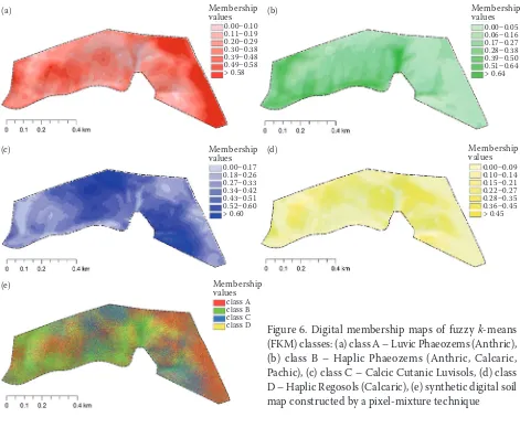
The classes A–D were interpolated into gridded membership maps with 5-m cell size. The four membership maps (Figures 6a–d) were rescaled as described in the methodology section to re-store the assumption of composite variables. The resultant pictures concur with field experiences. Luvic Phaeozems (class A) and Cutanic Luvisols (class C) occur especially at plateau parts of the study area where they represent the remnants of

Figure 6. Digital membership maps of fuzzy k-means (FKM) classes: (a) class A – Luvic Phaeozems (Anthric), (b) class B – Haplic Phaeozems (Anthric, Calcaric, Pachic), (c) class C – Calcic Cutanic Luvisols, (d) class D – Haplic Regosols (Calcaric), (e) synthetic digital soil map constructed by a pixel-mixture technique

Membership values

Membership values

Membership values

Membership values

Membership values

0.00–0.10 0.11–0.19 0.20–0.29 0.30–0.38 0.39–0.48 0.49–0.58 > 0.58

0.00–0.17 0.18–0.26 0.27–0.33 0.34–0.42 0.43–0.51 0.52–0.60 > 0.60

0.00–0.05 0.06–0.16 0.17–0.27 0.28–0.38 0.39–0.50 0.51–0.64 > 0.64

0.00–0.09 0.10–0.14 0.15–0.21 0.22–0.27 0.28–0.35 0.36–0.45 > 0.45

class A class B class C class D

(a) (b)

(c) (d)

a climax soil cover. Haplic Phaeozems of class B represent colluvial soils spreading along valleys, whereas Haplic Regosols of class D comprise erosive remnants of the former class A or C soils. Diffuse transitions between the four soil classes are visual-ized via the pixel-mixture method highlighted in Figure 6e. This kind of synthetic map can substi-tute for conventional soil maps and, moreover, it provides an intuitive picture of diffuse soil cover.

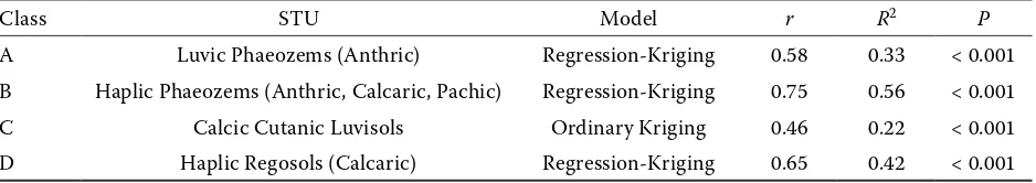
The four class membership maps were validated against the original MVs using the cross-validation approach (Table 4). The DSM model performed most effectively with class B and D MVs (R2 _= 56% and 42%, respectively, both P < 0.001). It per-formed less effectively, although still significantly with class A and C MVs (with R2 _{= 33% and 22%,} respectively, both P < 0.001).

CONCLUSIONS

The presented DSM model comprises FKM clas-sification and kriging of membership maps with the use of terrain predictors. The FKM method represents a formalized approach to soil classifica-tion which addresses the continuous character of soil objects. As shown above, the digitization of soil horizon properties gathered by way of con-ventional field observations provided reliable soil classes and MVs continuous enough to be spatially interpolated into membership maps. Resultant digital soil maps demonstrate a rational picture of the soil type distribution, which concur with expert field experience.

The DSM method was especially powerful for erosion-affected soil B and D classes where terrain variables significantly improved mapping perfor-mance. With a decreasing correlation between MVs and terrain variables, there was accompa-nying deterioration in DSM model performance.

The kriging component became more important for the spatial mapping of classes A and C, which were here located at plateau landscapes. Moreover, Cutanic Luvisols of class C are locally conditioned by the presence of clay stratum rather than the terrain alone, which was not considered by the DSM model. This is why the regression-kriging interpolation performed no better than the ordi-nary kriging method in this case.

Although the DSM model validity between 22 and 56% (P < 0.001) is not too high, it is worth noting that this study area is extremely heterogeneous due to the changes in erosion and accumulation processes over small distances. This is not fully captured even by this fine-scale sampling.

The spatial interpolation of MVs violates the compositional character of the fuzzy partition assumed by Eq. (1). Although this condition was formally restored by two-step rescaling of the re-sultant membership maps, this remains a methodi-cally suboptimal solution which could potentially benefit from the compositional kriging component introduced by Walvoort and De Gruijter (2001), once it is implemented to regression-kriging.

We conclude that the DSM model represents a completely formalized alternative to classical soil mapping at very small scales, even when the soil profile descriptions were collected merely by field estimation methods. Additionally to conventional soil maps, this model enables us to address the diffuse characteristics in soil cover, both in the taxonomic and geographical meanings. Here we must stress that the fine-scale soil inventories quickly emerge as a result of precise farming sup-port or environmental assessments at a municipal level. Increasing demands for soil information can be satisfied by local soil inventories supplying a significant and ever growing pool of soil informa-tion. Given that perspective, the coupling of such field surveys with remote sensing and GIS infor-Table 4.Cross-validation results; the relationships between original and modelled MVs were tested using linear regression (N = 111)

Class STU Model r R2 _P

A Luvic Phaeozems (Anthric) Regression-Kriging 0.58 0.33 < 0.001

B Haplic Phaeozems (Anthric, Calcaric, Pachic) Regression-Kriging 0.75 0.56 < 0.001

C Calcic Cutanic Luvisols Ordinary Kriging 0.46 0.22 < 0.001

D Haplic Regosols (Calcaric) Regression-Kriging 0.65 0.42 < 0.001

mation at fine scales will support the generation of important soil maps for farmers and executives.

Acknowledgements. This paper was financially supported by Ministry of Agriculture and Rural Development of the Slovak Republic in the Research Plan of the Soil Science and Conservation Research Institute (2011). We are very grateful to Ray Marshall for improving the English.

References

Ahmed S., De Marsily G. (1987): Comparison of geo-statistical methods for estimating transmission data on transmitivity and specific capacity. Water Resources Research, 23: 1717–1737.

Bezdek J.C., Ehrlich R., Full W. (1984): FCM: the fuzzy c-means clustering algorithm. Computers and Geoscienc-es, 10: 191–203.

Bourennane H., King D., Couturier A. (2000): Com-parison of kriging with external drift and simple linear regression for predicting soil horizon thickness with dif-ferent sample densities. Geoderma, 97: 255–271. Burgess T.M., Webster R. (1980): Optimal interpolation and

isarithmic mapping of soil properties. I. The semivariogram and punctual kriging. Journal of Soil Science, 31: 315–331. Burrough P.A., Van Gaans P.F.M., Hootsmans R. (1997): Continuous classification in soil survey: spatial correla-tion, confusion and boundaries. Geoderma, 77: 115–135. Carré F., Girard M.C. (2002): Quantitative mapping of soil

types based on regression kriging of taxonomic distances with landform and land cover attributes. Geoderma, 110: 241–263.

De Gruijter J.J., McBratney A.B. (1988): A modified fuzzy k-means for predictive classification. In: Bock H.H. (ed.): Classification and Related Methods of Data Analysis. Elsevier Science, Amsterdam, 97–104.

De Gruijter J.J., Walvoort D.J.J, Van Gaans P.F.M. (1997): Continuous soil maps – a fuzzy set approach to bridge the gaps between aggregation levels of process and distribution models. Geoderma, 77: 169–195.

FAO-ISRIC-ISSS (2006): World Reference Base for Soil Re-sources. World Soil Resources Report No. 103, FAO, Rome. Gobin A., Campling P., Feyen J. (2001): Soil-landscape

modelling to quantify spatial variability of soil texture. Physics and Chemistry of the Earth. Part B: Hydrology, Oceans and Atmosphere, 26: 41–45.

Goovaerts P. (1999): Using elevation to aid the geostatis-tical mapping of rainfall erosivity. Catena, 34: 227–242. Hengl T., Heuvelink G.M.B., Stein A. (2004a): A generic

framework for spatial prediction of soil variables based on regression-kriging. Geoderma, 120: 75–93.

Hengl T., Walvoort D.J.J., Brown A. (2004b): A double continuous approach to visualisation and analysis of categorical maps. International Journal of Geographical Information Science, 18: 183–202.

Johnston K., Ver Hoef J.M., Krivoruchko K., Lucas N. (2001): Using ArcGIS Geostatistical Analyst. GIS by ESRI, Redlands.

Kalivas D.P., Triantakonstantis D.P., Kollias V.J. (2002): Spatial prediction of two soil properties using topographic information. Global Nest: the International Journal, 4: 41–49.

Knotters M., Brus D., Voshaar J. (1995): A comparison of kriging, co-kriging and kriging combined with regres-sion for spatial interpolation of horizon depth with cen-sored observations. Geoderma, 67: 227–246.

Lagacherie P. (2005): An algorithm for fuzzy pattern matching to allocate soil individuals to pre-existing soil classes. Geoderma, 128: 274–288.

Maidment D.R. (2002): Arc Hydro: GIS for Water Re-sources. ESRI Press, Redlands.

McBratney A.B., Moore A.W. (1985): Application of fuzzy sets to climatic classification. Agricultural and Forest Meteorology, 35: 165–185.

McBratney A.B., De Gruitjer J.J. (1992): A continuum approach to soil classification by modified fuzzy k-means with extragrades. Journal of Soil Science, 43: 159–175. McBratney A.B., Mendonça Santos M.L., Minasny B.

(2003): On digital soil mapping. Geoderma, 117: 3–52. McKenzie N.J., Ryan P.J. (1999): Spatial prediction of soil

properties using environmental correlation. Geoderma,

89: 67–94.

Melville M.D., Atkinson G. (1985): Soil color: Its meas-urements and its designation in models of unifoem color space. Journal of Soil Science, 36: 495–512.

Minasny B., McBratney A.B. (2002): FuzME Version 3. Australian Centre for Precision Agriculture, University of Sydney, Sydney.

Moore I.D., Grayson R.B., Landson A.R. (1991): Digital terrain modelling: A review of hydrological, geomor-phological, and biological applications. Hydrological Processes, 5: 3–30.

Odeh I.O.A., McBratney A.B., Chittleborough D.J. (1994): Spatial prediction of soil properties from land-form attributes derived from a digital elevation model. Geoderma, 63: 197–214.

Odeh I.O.A., McBratney A.B., Chittleborough D.J. (1995): Further results on prediction of soil properties from terrain attributes: heterotopic cokriging and re-gression-kriging. Geoderma, 67: 215–226.

Schoeneberger P.J., Wysocki D.A., Benham E.C., Broderson W.D. (2002): Field book for describing and sampling soils, Version 2.0. Natural Resources Conserva-tion Service, NaConserva-tional Soil Survey Center, Lincoln. StatSoft Inc. (2003): STATISTICA (Data Analysis Software

System), Version 6. Tulsa. Available at www.statsoft.com ter Braak C.J.F., Šmilauer P. (2002): CANOCO Refer-ence Manual and CanoDraw for Windows User’s Guide: Software for Canonical Community Ordination (Ver-sion 4.5). Ithaca.

Walvoort D.J.J., De Gruijter J.J. (2001): Compositional kriging: A spatial interpolation method for compositional data. Mathematical Geology, 33: 951–966.

Webster R., Oliver M.A. (2007): Geostatistics for Envi-ronmental Scientists (Statistics in Practice). 2nd _{Ed. John} Wiley & Sons, Padstow.

Wilson J.P., Gallant J.C. (2000): Terrain Analysis: Prin-ciples and Applications. John Wiley & Sons, New York. Zádorová T., Penížek V., Šefrna L., Rohošková M.,

Borůvka L. (2011): Spatial delineation of organic car-bon-rich Colluvial soils in Chernozem regions by Terrain analysis and fuzzy classification. Catena, 85: 22–33. Zhu A.X., Hudson B., Burt J., Lubich K., Simonson D.

(2001): Soil mapping using GIS, expert knowledge, and fuzzy logic. Soil Science Society of America Journal, 65: 1463–1472.

Received for publication August 14, 2012 Accepted after corrections November 12, 2012

Corresponding author

RNDr. Juraj Balkovič, PhD., International Institute for Applied Systems Analysis, Schlossplatz 1, A-2361 Laxenburg, Austria