Characterisation and description of compressible rubbery materials for component modelling

1

Characterisation and Description of Compressible

Rubbery Materials for Component Modelling

Nathan Townsend

A dissertation submitted in partial fulfilment of the requirements for the

degree of MPhil

Department of Engineering, Design and Mathematics, University of the

West of England, Bristol

2 ABSTRACT

Rubbery foams and similar highly compressible rubbery solids form an important class of materials for technology. In order for components made from such materials to be modelled, in Finite Element Analysis (FEA) for example, appropriate constitutive laws are required. The review of the literature revealed that rubbery foams lacked the array of comprehensive data sets that have been published for near-incompressible rubbery materials for example. Moreover there were important contradictions between accounts of how rubbery foams behaved at finite strains. The review of the literature also raised some doubts on what the value of Poisson’s ratio (ν) should be for such materials in simple extension – let alone in compression.

Most finite strain FEA of rubbery foams seems to use in the constitutive law a finite strain version of ν based on logarithmic strains: here called the Poisson index, υ. Some of the implications of such approaches have been explored via theory and experiments. Some doubt has thereby been cast on such approaches.

3 Table of contents

ABSTRACT

1. INTRODUCTION

2LITERATURE REVIEW

2.1 Elasticity at infinitesimal strains and the Poisson ratio (ν) 2.2 Finite deformations

2.2.1 Measures of finite deformation

2.2.2 Modelling of elastic behaviour at finite strain and the definition of the Poisson index (υ)

2.3 Forms of constitutive law for rubbery materials – treated as isotropic and elastic up to large strains

2.3.1 Rubbery materials without voids

2.3.2 Rubbery foams and other highly compressible materials 2.4 Existing sets of data for rubbery foam and micromechanical models 2.5 The work of Chagnon & Coveney (2008, 2011)

2.6 General discussion

3RESEARCH QUESTIONS, AIMS, OBJECTIVES & PLAN OF WORK

3.1 Key points from literature review in relation to this piece of work 3.2 Research questions arising

3.3 Aims, objectives & plan of work 4THEORY

4.1 Loci in I₁,I₂,Jspace, for constant Poisson index (), of various modes of deformation

4.2 Generalisation of Blatz & Ko’s approach and behaviour in specific modes of deformation

4.2.1 Generalisation of Blatz & Ko’s approach

4.2.2 Simple uniaxial extension and compression (SE/C) 4.2.3 Equibiaxial extension/compression (EBE/C) 4.2.4 Fixed width extension/compression (FWE/C)

4.2.5 Constant cross-section, or plane, extension/compression 4.2.6 Pure volume change

4.2.7Simple shear

4.3 Further experimental test options considered

4 5EXPERIMENTAL WORK

5.1 Materials for experiments 5.1.1 Introduction

5.1.2 Measurement of the density of the natural rubber latex foam 5.1.3 Finding the volume fraction of rubber in the foam

5.1.4 Finding the volume fraction of closed cells in the foam

5.1.5 Removal of “skin” from the Pentonville Foam natural rubber latex foam 5.1.6 Conditioning of the test piece

5.2 Simple shear test

5.2.1 Apparatus and experimental procedure 5.2.2 Results and discussion for simple shear test 5.3 Simple extension tests

5.3.1 Apparatus

5.3.2 Deformation measurement 5.3.3 Experimental procedure. 5.4 Simple compression tests

5.4.1 Apparatus and procedures

5.4.2 Results and discussion for simple extension and compression tests 5.5 Pressure-volume tests

5.5.1 Apparatus and procedures 5.5.2 Experimental method

5 6CONCLUSIONS &RECOMMENDATIONS

APPENDIX I. SMALL STRAIN ELASTICITY

APPENDIX II DESCRIPTION OF TESTING METHODS

APPENDIX III MEASURES OF DEFORMATION FOR FINITE DEFORMATION APPENDIX IV STRESS AT FINITE DEFORMATION

Calculating stress from derivatives of the strain energy density

APPENDIX V STRESS PREDICTIONS FOR A GENERALISED BLATZ &KO (GBK) AND OTHER FORMS

V.1 Cases of pure homogeneous strain for a generalised Blatz & Ko (GBK) and other materials

V.1.1 Simple extension/compression (SE/C) V.1.2 Equibiaxial extension/compression (EBE/C) V.1.3 Fixed width extension/compression (FWE/C) V.1.4 Constant cross-section extension/compression V.1.5 Pure volume change

6 LIST OF FIGURES

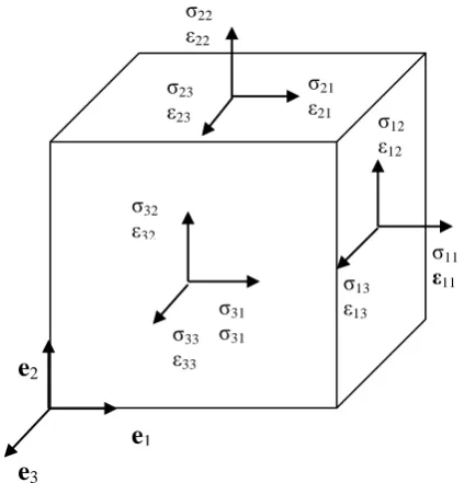
Figure 1. Unit vectors in the 1, 2 and 3 directions and conventional strain εij and stress σij

components for a cuboid of material.

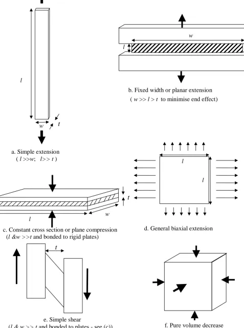
Figure 2. Modes of test for material properties (schematic)

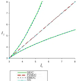
Figure 3. Loci of simple extension/compression(SE/C), equibiaxial extension/compression (EBE/C), fixed width extension/compression(FWE/C) and simple shear (SS) for an

incompressible material on the I1, I2 plane.

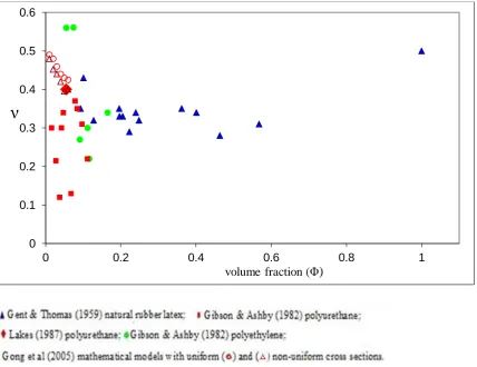
Figure 4. Poisson’s ratio ( ) versus volume fraction (Φ)for a range of foams.

Figures 5.a to g showing loci for simple extension and compression (SE/C), equibiaxial extension and compression (EBE/C) fixed width extension and compression (FWE/C) and simple shear (SS) for

υ

=

-0.75, -1.

Figure 6. Simple shear: a material point at P in the undeformed condition moves to P’. Figure 7. Pentonville Foam natural rubber latex foam with mm rule to show scale of cells. Figure 8. Simple shear test apparatus.

Figure 9. Diagram illustrating simple shear test piece comprising natural rubber latex foam . Figure 10. Simple shear; Shear strain γ = tanθ.

Figure 11. Plots of

𝜎

𝜎

Figure 12. Simple extension test piece, grips and coordinate system. Figure 13. (a) and (b) Details of upper and lower pointers and mm scale. Figure 14. Side view of tapered wooden grip holding foam test piece. Figure 15. Details of arrangement of central markers.

Figure 16. Detail of rigid aluminium strut used to offset upper grip. Figure 17. Apparatus for simple compression test.

Figure 18. Simple compression test (a) λ1 = 1 (b) λ1 = 0.7 (c) λ1 = 0.4 (d) coordinate system. Figure 19. Nominal stress (1,1 component N) against extension ratio (λ1).

Figure 20. Lateral Hencky (lnλ2) strain against longitudinal Hencky strain (lnλ1).

Figure 21. Poisson index (υ) versus lnλ1.

Figure 22. Cork filled polyurethanes (a) PR1, (b) PR5.

Figure 23. Photograph of the pressure chamber in situ, showing fibre-optic lights etc. Figure 24

.

Figure 25. Typical image showing part of dilatometer tube.

Figure 26. Plot of pressure against fractional decrease in volume (1-J) for cork filled polyurethane, PR1.

Figure 27. Plot of pressure against fractional decrease in volume (1-J) for cork filled polyurethane, PR5.

7

Acknowledgements

I would like to thank everyone who has helped, encouraged and supported me throughout the years I have spent studying for my MPhil.

In particular I would like to express my sincere gratitude to my director of studies Dr VA Coveney for all his tireless effort, support and encouragement.

Special thanks also to Dr G Chagnon whose work with Dr VA Coveney was referred to throughout this study.

I would also like to thank Professor M Smith for help and support as director of studies during the final years of this study.

Thanks also to my additional supervisor Dr A Farooq for offering help and advice when needed.

8 1. INTRODUCTION

This project focuses on highly compressible materials, mainly rubbery foams, and the constitutive models used to describe these. Rubbery foams are important materials and widely used in health, transport and many other technical areas. Their functions include shock and impact reduction, noise absorption and isolation from vibration.

Rubbery materials without voids can undergo large strains of hundreds of percent in tension as well as in compression more or less elastically. For materials without voids the shear modulus (μ) is ~1 MPa, whereas the bulk modulus (K) is ~2 GPa.

Because K/ μ is so high these materials have Poisson ratios close to ½ and are sometimes called near incompressible.

Voided or cellular rubbery solids otherwise known simply as rubbery foams have shear moduli that are generally lower and bulk moduli much lower than those for solid rubbers. Foam materials can have open or closed cells with geometry that can be either regular or irregular. They can be composites, with hollow or otherwise highly compressible inclusions e.g. cork. The single most important feature of a rubbery foam material is the fraction of the volume occupied by solid rather than air or another gas. This is the volume fraction (Φ) of the foam; provided the density of the gas can be ignored it is equal to the density of the cellular material divided by the density of the solid from which it is formed, ρ /ρS . Ultra low density foams can have a volume fraction as low as 0.001. General purpose polymeric foams have a volume fraction of between 0.05 and 0.2. A foam material is normally described as having a volume fraction of below about 0.3. Above this value the dense foam is sometimes described as a solid containing isolated pores (Gibson & Ashby, 1997).

Foam materials are especially good at absorbing energy in impacts while keeping the peak force below a level that would cause damage. They will always give a lower peak force than a non-foam solid of the matrix material (Gibson & Ashby, 1997). The buckling and collapse of cells can allow a large amount of energy to be absorbed at a near constant load (Gibson & Ashby, 1997). A number of mechanisms can be at work when a foam is absorbing energy. Some relate to the elastic deformation of the cells while others depend on the compression or flow of the fluid within the cell walls (Gibson & Ashby, 1997). So the behaviour of a

particular foam depends on the cell wall material; it also depends on whether there are open cells so that they are interlinked or closed cells so that the cells are isolated (Schwaber, 1973). In order for rubbery foams have component modelling done in Finite Element Analysis for example, appropriate constitutive laws are required. Such material models usually need to describe elastic behaviour up to large deformations; this is the principal subject of the present work. Such constitutive laws should give physically plausible and accurate stress and

dimensional changes for a wide variety and range of deformations in compression and tension up to around 100% strain. A material needs to be characterised throughout a wide range of modes of deformation and combinations of these modes in order to properly simulate conditions a component will encounter. For example a seat cushion will be subject to compression but will also experience deformation in tension at the edges of the loaded area. Published data up to these large strains for rubbery foam is limited and often of

9

extension and compression experiments on natural rubber foams. More recently tests were carried out on two types of polyurethane foam by El-Ratal & Mallick (1996), Mills &

Gilchrist (1997) also tested polyurethane foam. The same authors also attempted macroscopic modelling of foams. Gibson & Ashby (1997) carried out extensive work on rubbery foams and many other related cellular solids including cork, wood and bone.

10 2 LITERATURE REVIEW

The main subject of the current dissertation is the behaviour of isotropic compressible elastic materials at finite strains, however any valid model of the behaviour of such materials must correspond to an infinitesimal strain model at such strains.

2.1 Elasticity at infinitesimal strains and the Poisson ratio (ν)

At infinitesimal strains in linear elastic materials, stresses are proportional to strains. Please see Figure 1.

Figure 1. Unit vectors in the 1, 2 and 3 directions and conventional strain εij and stress σij

components for a cuboid of material.

Linear elastic, isotropic solids, Hookean or Lamé solids, are characterised, at infinitesimal strains, by any two of the elastic constants: ,,K,Eand  (the 1st Lamé constant, the 2nd Lamé constant or shear modulus, the bulk modulus, the Young modulus and the Poisson ratio). The constants relate stresses to strains; the Poisson ratio can also be used to relate principal strains (_i) to each other. The Poisson ratio is best known for relating lateral strain to simple extension; more generally gives the strain in the 3rd direction if the other two strains are specified in general biaxial strain under plane stress conditions. Consider a cuboid of material aligned with the direction of principal strain (so that _ij= 0, i ≠ j) if ₁₁ and ₂₂are applied and faces in the 3 direction are stress free,₃₃ (i.e.₃) is given by

) (

1 1 2

3 _  



 

 

 (2.1)

(See Mars, 2006 and Appendix I.)

Schematic examples of modes of test are shown in Figure 2 and Appendix II .

σ22

ε22

σ23

ε23

σ21

ε21 _σ 12

ε12

σ32

ε32

σ11

ε11

σ13

ε13

σ31

σ31

σ33

ε33 e2

e1

11

l

( w >> l > t to minimise end effect)

c. Constant cross section or plane compression (l &w >>t and bonded to rigid plates)

d. General biaxial extension

e. Simple shear

(l & w >> t and bonded to plates - see (c))

l

l

a. Simple extension ( l >>w; l>>t )

w

l

b. Fixed width or planar extension

t w

w

f. Pure volume decrease

Figure 2. Modes of test for material properties (schematic)

t

t

l

12

Although most solids have Poisson ratios of around 0.3, -1 < ν < ½ is generally accepted as being the permissible range in principle for isotropic solids (Mott & Roland, 2009 and 2013; Greaves et al, 2011); K falls to zero at the lower limit and rises towards infinity at the upper. Clearly, neither the lower nor the upper limit can be reached for any real material,

nevertheless the upper limit gives an idealisation widely-used in rubber modelling (Treloar, 1975; Rivlin, 1992). The range 0 ≤ ν < ½ corresponds to “non-auxetic” and -1 < ν < 0 to “auxetic” behaviour - see Gibson & Ashby (1997) and Alderson & Evans (1997) for

example). By considering several modes deformation Mott & Roland (2009 and 2013) argue that the non-auxetic range should be further divided and that all normal isotropic elastic solids, to which the Lamé framework of elasticity is applicable, have 1/5 ≤ ν < ½. 2.2 Finite deformations

2.2.1 Measures of finite deformation

In what follows F is the deformation gradient ∂x/∂X or

j i ij

X x F

 

 in component form (Holtzapfel, 2000; Bower, 2009); X and x are material and spatial coordinates respectively – corresponding to the reference configuration and the current configuration .

For isotropic materials that are elastic up to finite strains, deformation is usually measured using one of the following (Rivlin, 1992; Holzapfel 2000; Treloar 1976).

(a) The principal scalar invariants (I₁,I₂,I₃) of the Cauchy-Green deformation tensor, right (C) or, here, left (B, sometimes written b); Holtzapfel (2000), Oden (1972, 2000), Rivlin (1992), Bower, 2009.

(b) The eigenvalues (₁2,2₂,2₃) of B (or C) or their square roots, the principal extension ratios or stretches (Eihlers & Eipper, 1998; Storåckers, 1986; Bruhns et al, 2001; Bower, 2009).

(c) Simple rearrangements of (a) such as the volume ratioJ  I₃ and invariants of “volume

neutralised” B and C, BJ2/3BandCJ2/3C i.e. invariants modified to remain

unchanged for pure volume change (I₁ and I₂) – see Penn (1970), Treloar (1975), Ehlers & Eipper (1998), Gough et al (1999) or Bower (2009) for example. (d) Simple rearrangements of (b) such as the natural logarithmic or Hencky strains (principal values e_i ln_i) or the volume neutralised principal extension ratios (Simo & Taylor, 1991; Gough et al, 1999; Bruhns et al, 2001).

13

2.2.2 Modelling of elastic behaviour at finite strain and the definition of the Poisson index (υ)

What is called herein the Poisson index (υ) is a finite strain version of the Poisson ratio relating logarithmic strains (e_i ln_i) – please see Blatz & Ko, 1962; Ogden, 1972a). As Ogden (1972b) points out, υ will, in general, be a function of the deformation – see also: Alderson et al (1997); Pierron, 2010). There is disagreement between various authors on the extent to which υ varies with deformation of rubbery foams; some workers indicate that υ

varies little if at all with extension (Blatz & Ko, 1962; Storåckers, 1986 ) – others indicate that υ varies by a surprisingly large amount: El-Ratal & Mallick (1996) and see later in this dissertation.

Using Kirchoff stress (Bruhns et al, 2001) some authors use the direct Hencky, (1928) approach to extend the equations of isotropic elasticity at infinitesimal strain to calculate the stresses at finite strains via logarithmic strain (ei). ei ln

 

the Blatz & Ko form of constitutive law (please see below and Blatz & Ko, 1962) or Ogden’s model that has come to be known as the hyperfoam model as usually implemented also use the Poisson index (υ) and assume that it can be regarded as a constant (Storåckers, 1986.). Chagnon & Coveney (2008, 2011) argue that irrespective of whether υ is constant or not, it can be defined for a particular state of strain, if faces in the 3 direction are stress free, by





1 1 2

3 e e

e 

  

  or





3 

  

 

 

Please see Figure 1.

It should be noted, though, that such a definition hypothesises that aspects of the Hencky (1928) approach are appropriate for the material being modelled.

14

2.3 Forms of constitutive law for rubbery materials – treated as isotropic and elastic up to large strains

2.3.1 Rubbery materials without voids

Solid rubbery materials are described as near incompressible because the bulk modulus (K) is very large compared with the shear modulus (μ). It is usual to assume that a Helmoltz free energy function (W) of the deformation gradient (F) can be used to describe them:

 

W W 

W, also known as the strain energy density, is defined per unit volume in the reference configuration (Rivlin, 1992; Gough et al, 1999; Holtzapfel, 2006). Treating rubber as incompressible, Rivlin (1948, 1992) used symmetry to argue that because W is a function of the deformation gradient it must also be a function of the first two principal invariants of the left or the right Cauchy-Green deformation tensor B or C:





W 

So the current view is that the strain energy density of any isotropic elastic incompressible material can be described by equation 2.4 and the stresses found from its derivatives – as explained by Rivlin (1948, 1992), Rivlin & Sawyers (1976), Holzapfel (2006), Bower (2009) and elsewhere.

Maclaurin expansion gives what has come to be known as the Rivlin series form of constitutive law (Rivlin & Saunders, 1951):



 



ij I I

C

W 



If ∂W/∂I1 and ∂W/∂I2 are taken to be constants C10 = C1 and C01 = C2 respectively, equation

2.5 simplifies to the Mooney, or Mooney-Rivlin, form:









1   

C I C I

W

Here 2C1 + 2C2 = μ, the shear modulus. If ∂W/∂I2 is taken to be zero, equation 2.6 simplifies

to the neo-Hookean form (Treloar, 1975):





 I

W 

Equation 2.7 is also given by the Gaussian statistical theory of rubber elasticity with μ proportional to absolute temperature (Treloar, 1975). In the neo-Hookean form, the stresses associated with shape changes are calculated with knowledge of just one material constant: the shear modulus μ – as is the case at infinitesimal strains.

15

problems, the fitting of these experimental results by an algebraic expression for W is, in large measure, an empty exercise… Indeed, if the solution of the problem involves the use of a computer, one could just as well take the experimentally determined dependence of ∂W/∂I1

and ∂W/∂I2 on I1 and I2 as a constitutive input to the problem.”

The experimental investigation of how ∂W/∂I1 and ∂W/∂I2 dependon I1 and I2 has centred on

general biaxial extension of sheets of rubber in the plane stress condition (see Figure 2). Treloar (1975) shows, for an incompressible material, the loci of simple extension

/compression, equibiaxial extension/compression and fixed width extension/compression on the I1, I2 plane. The loci are replotted in Figure 3. The curves of simple extension

/compression and equibiaxial extension/compression give the boundaries of what are possible values of I1, and I2 for general biaxial extension. Note that, as expected the loci for simple

extension/compression, equibiaxial extension/compression merge in to that for fixed width extension/compression as the values of I1 and I2 approach 3.

Figure 3. Loci of simple extension/compression (SE/C), equibiaxial

extension/compression(EBE/C), fixed width extension/compression(FWE/C) and simple shear (SS) for an incompressible material on the I1, I2 plane.

Gent & Rivlin (1951), Rivlin (1992) and Gough et al (1999) have discussed the experimental evidence on how W or rather ∂W/∂I1 and ∂W/∂I2 for rubbery materials without voids depend

on I1 and I2. All three publications make it clear that wherever it is possible to distinguish

well between ∂W/∂I1 and ∂W/∂I2, because strains are sufficiently large, ∂W/∂I1 is at least five

times larger than ∂W/∂I2. Gent & Rivlin (1951) suggest, on the basis of their data and the data

of others, that ∂W/∂I2 is associated with energy dissipation and speculate that structurally it

may be associated with some form of secondary, relatively fragile reformable, crosslinks. Kawabata (1973) performed plane stress general biaxial measurements on natural rubber and SBR (styrene-butadiene rubber) materials over a temperature range of 20 to 100 °C. He found that ∂W/∂I1 was approximately proportional to absolute temperature (see equation 2.7) but

3 4 5 6 7 8

3 4 5 6 7 8

I1

I2

16

that ∂W/∂I2 was substantially temperature independent. He found that the relaxation

behaviour of ∂W/∂I2 closely resembled that of ∂W/∂I1 and that the relaxation time was almost

the same.

Gough et al (1999) warned that the common practice of applying conditioning cycles of deformation to a test piece may produce anisotropy. They say that their data and the data of others for a number of practical rubbery materials is consistent with ∂W/∂I2 being zero but not

for one material. They point out that when strains are insufficiently large it is no longer possible to distinguish between I1 and I2.

Edwards & Vilgis (1986) have proposed modifying the Gaussian statistical theory of rubber elasticity to allow for chain slippage at small strains and to account for stiffening at large strains via the tube concept.

Because the role of ∂W/∂I2 is, at most, less important than that of ∂W/∂I1 in rubber elasticity

and because dropping ∂W/∂I2 in a model gives benefits, a number of authors have decided to

do this, including: Yeoh (1990), Arruda & Boyce (1993), Davies et al (1994), Gent (1996) and Marlow (2003) who proposes direct use of experimental results for W(I1) in finite

element analysis. Some of these approaches seem to work well – see Boyce & Arruda (2000) for example.

A number of authors, including Mooney (1940), Carmichael & Holdaway (1961) and Valanis & Landel (1967) have hypothesised that W can be expressed as a sum of functions of the principal extension ratios, or their squares:

     

w

W   

Rivlin & Sawyers (1976) showed that forms of W conforming to equation 2.8, the “Valanis- Landel” hypothesis, imply that the dependence of W onI₁andI₂conforms to the following:

) 9 2 (

2 1

2 2 2 2 2

2 2

1 2 1 2 1 2

1

. I

I W I

I W I

I I

W I I

W

I _

 

 

 

    

      

 

 

    



As pointed out by Gough et al (1999) strain energy density functions conforming to the Valanis-Landel hypothesis have “been found to work well in practice, at least for unfilled rubber up to moderately large strains [by] Obata et al, 1970; Valanis & Landel, 1967; Jones & Treloar, 1975; Ogden, 1972”. However, they go on to point out that Gent’s (1996) strain energy density function (designed for use up to high strains) does not conform to equation (2.9). The same will be true of any strain energy density function which has ∂W/∂I2 ≡ 0 but

which includes high powers of I1 .

w in equation 2.8 may, in turn, be expanded as a series of integer powers of λi (Mooney, 1940) or as a general power series (Ogden, 1972a):







 ₁i ₂i ₃i 3

i i

W   

 

(2.10)

Here the powers, αi can be have any real value. Note that some authors use eigenvalues of B

17

If there is still debate about the possible role of I2 and its origin and about the suitability of

the Valanis-Landel hypothesis there is further debate about how best to represent the compressibility of rubbery materials without voids.

If the ideal, isotropic elastic material is compressible, equation 2.3 gives (Rivlin, 1992; Bower, 2009)





W

W 

[note that the use of W on the right hand of each of equations 2.3, 2.4, 2.11a, 2.11b means that the strain energy density is a function of the variables written but not that the functional is the same in each case.]

or equivalently, but with different Cijk





W

W 

Maclaurin series expansion gives (Oden, 1972, 2000):



 

 



k j

i

ijk I I I

C

W 



or equivalently



 







k j

i

ijk I I J

C

W 



The Cauchy stress can be found by using a formula such as the following – see Appendix IV or Chagnon (2003) or Bower (2009) for example:

I I

B B I

B σ

J W I

W I

I J I W I

J 

      

 _{ }

     

  

2 2 2 1

1 1

3 2 2

3 1 2

(2.13)

Rivlin (1992) emphasises the difficulty in experimental determination for equations 2.11 or 2.12 if there are no simplifications; this is because W/I₁,W/I₂andW/Jcan each be functions of I₁,I₂ andJ. A widely used simplification suggested by Flory (1960; see also Gough et al, 1999) is to separate W into an isochoric part purely due to shape change (Ws) and a dilational part purely due to volume change (Wv):





 

W  s  v

or equivalently





 

W  s    v

used. be can of

any two that

so 1 that

18

Forms conforming to equation 2.14(a)can be called shape-volume uncoupled – e.g. in equation 2.14 Wv /I1 Wv /I2 Ws /J 0.

Blatz & Ko (1962) put forward the following form that is a modification of the Mooney form (equation 2.6) allowing for compressibility via a constant Poisson index (υ):









1

3 2 1 2

2 2 2 2

1 2 1

1 J .

J I C J

I C

W /( ) /( )

  

  _

  

  

  _

 

     

  



where C1 + C2 = μ/2 – please see Treloar (1975) and equations 4.2.2 and 4.2.18.

The volume neutralised principal invariants are

can write we

so

and ₂ 4 3 ₂

1 3 2

1 J I I J I

I   /   /











 _{ }  _

   

 _{ }  _

    

1 2

1 3

1 2

1

3 2 2 1 2

3 4 2 2 2

1 2 1

3 2 1

) /( /

) /( /

J I

J J C J

I J C

W    

  



or

(2.16) 1

2 1 3 1

2 1

3 1 2

2

2 3 2 2 2

1 2

1 3 2 1

    

  

    

  

 

  

    

  

    

  

 

 

   



  



  



J I

J C J

I J C

W / /

Equation 2.16 shows the Blatz & Ko equation in a way that emphasises that there is a particular sort of coupling between shape changes and volume changes in the calculation of

W.

Penn (1970) measured volume change of rubber in simple extension and found that the results were not consistent with shape-volume separation in the strain energy density

(equation 2.14). Ogden (1972b) referred to Penn’s work (1970) to argue in favour of the type of shape-volume coupling used in the Blatz & Ko model (equation 2.16). Gough et al (1999) however said that the experimental errors in Penn’s (1970) measurements of volume change were such that shape-volume separation could not be refuted on the basis of his data. They do, though, argue for a form of Wv that is an uneven function of (J-1) and that “rises towards

infinity as it must when the volume approaches zero”. Ehlers & Eipper (1998) on the other hand find that shape-volume uncoupled models can lead to unrealistic behaviour with cross-section increasing at high degrees of simple extension and decreasing at high degrees of simple compression. The volume of natural rubber increases slightly at simple extensions up to about 100% but decreases at strains of hundreds of percent, because of crystallisation, where the nominal Poisson index will therefore exceed ½ (Ogden, 1972b; Treloar, 1975). According to Ogden (1972b) at λ1 = 8, J = 0.98

Now J = λ1 λ2 λ3 = λ λ-υ λ-υ = λ1-2υ 0.505 (2.17)

ln ln 1 2 1



  

    



19

2.3.2 Rubbery foams and other highly compressible materials

If there is some question about whether shape-volume coupling is necessary for rubbery materials without voids, for highly compressible rubbery materials (e.g. rubbery foams) shape-volume coupling seems difficult to argue against – especially if they are likely to undergo large deformation in compression as well as in extension. Equations 2.11 and 2.12 show the general descriptions but, as stated above, consideration of the dependence of W, or its three derivatives, in I₁,I₂ andJ space would be a major undertaking, perhaps because of this, the Blatz & Ko form (equations 2.15 and 2.16) and what is now known as the hyperfoam form (Ogden, 1972b; Hill, 1978; Storåckers, 1986; Mills & Gilchrist, 2000a)

















 

i i i

i

i i

i _J i i i i _J i i

W 2 ₂  /3 ₁ ₂ ₃ 3 2₂  1

 

 

  



(2.18)

are widely used. Of the constants, _i and _i can take any real value, the initial shear modulus



 i

i





i i

i _

 

2 1

 so multiple constant (sub) Poisson indices can, in principle, coexist. However, in practice, a single constant Poisson index is generally chosen

(Storåckers, 1986; Mills & Gilchrist, 2000a and see below). It can be seen that the hyperfoam form is a generalisation of the Blatz & Ko form – please see equation 2.16 and Storåckers (1986) for example.

2.4 Existing sets of data for rubbery foam and micromechanical models

Blatz & Ko (1962), Blatz (1963) tested a polyurethane rubbery foam - or rubbery solid with pores - with a fraction of rubber by volume of the foam (Φ) of 0.53; unlike some

polyurethane foams this one was more likely to be isotropic because of the way it was made (Blatz & Ko, 1962; Gibson & Ashby, 1997). The material was tested in simple, equibiaxial and fixed-width extensions. Their method implied that equation 2.2 was being used. Their data shows little scatter and a value of υ = 0.25 was obtained, by means of particularisations of equation 2.2. After having decided that υ should be 0.25 Blatz & Ko went on to compare the stresses given by their equation (equation 2.15) to the measured stresses. They came to the surprising conclusion from this comparison that C1 in equation 2.15 was small and could

be ignored and so arrived at what has come to be known as the Blatz-Ko form of strain energy density function implemented in some commercial Finite Element Analysis software (Bower, 2009).

Storåckers (1986) questioned the results of Blatz & Ko (1962) and obtained υ = 0.32 from for simple, equibiaxial and fixed-width extension of a natural rubber (NR) foam and υ = 0.49 for (b) an EPDM (ethylene-propylene-diene) rubber foam. His method implied that equation 2.2 was being used. The value of υ for NR foam is well within the expected range but the value for the EPDM foam seems high. Storåckers said only that the NR foam was highly

20

Gent & Thomas (1959, 1963) described a simple micromechanical model, for an idealised open cell rubbery foam, of strands of rubber; a Poisson ratio (ν) of ¼ was predicted. They performed simple (uniaxial) extension experiments on 15 natural rubber latex foams of volume fractions (rubber volume divided by foam volume) Φ varying from 0.093 to 0.568, checking that the rubber matrices were all similar. The method of manufacture of the foams meant that the foams were likely to be essentially isotropic (Gent & Thomas,1959,

1963).They measured ν at about 10% simple extension as 0.33 0.04; their set of data suggested that ν did not vary with Φ. Gibson & Ashby (1982) described a relatively simple micro-mechanical model for open and closed cell foams. Gibson & Ashby’s model, based on bending of members, predicted a ν of 0.33. The experimental results of Gent & Thomas (1959, 1963), Gibson & Ashby (1982, 1997) and others covering a very wide range of Φ together with the model of Gibson & Ashby pointed to ν for open and closed cell foams varying little for “all values” of Φ, i.e. up to Φ = 0.6 at least; the combined experimental results Gibson & Ashby (1982, 1997) presented showed considerable scatter but “there is no systematic variation with density [relative density i.e. Φ]..The average value is about 1/3.” A graph summarising published experimental data for ν against Φ is shown in Figure 4. Some of Gibson & Ashby’s (1982) results fell outside the range of ν for normal materials, but they did not comment on this. They did not state at what strain or strains they made the Poisson ratio measurements.

Results presented by Gent & Thomas (1959) included plots of, presumed, nominal stress against engineering strain (ε =λ - 1) in simple extension and also for, nominal, simple compression for test pieces of natural rubber latex foam of 0.125. λ was from 0.6 to 1.15. The plot of stress against λ is essentially linear in extension but shows a sudden drop in tangential stiffness (slope of the graph) at small compressive strain (i.e. between λ ≈ 1 and 0.97). Such behaviour is thought to be associated with the onset of buckling of the cell walls or ligaments in the foam (Gent & Thomas, 1959; Gibson & Ashby, 1997).

There have been many publications on attempts at micromechanical modelling of rubbery foam since 1963, Gong et al (2005a&b) reviewed some of this work as well as producing their own micromechanical models of increasing complexity and performing some physical experiments – unfortunately all the experiments were on anisotropic foams. It is noted that the modelling results of Gong et al (2005a) for isotropic foam predicted that ν will tend towards 0.5 as Φ tends towards zero (please see Figure 4). Gan et al (2005) have also

reviewed micromechanical modelling of solid foam and also produced a model that predicted that ν will tend towards 0.5 as Φ tends towards zero. Neither sets of authors commented on the fact that this prediction differed from the predictions of other models and from what most of the published experimental data seem to show.

21

Figure 4. Poisson’s ratio ( ) versus volume fraction (Φ)for a range of real and modelled foams.

As indicated above, Blatz & Ko (1962) and Storåckers (1986) found that υ did not vary with simple extension, equibiaxial extension and fixed width deformation. El-Ratal & Mallick (1996) performed simple extension tests on (a) a “seat foam” and (b) a “commercial foam” – both polyurethane. For foam (a) they found that υ at λ = 1.1 was about 0.25 but

at λ = 1.4, υ was approximately 0.6. For foam (b) υ at λ = 1.1 was about 0.35 but at λ = 1.4, υ was approximately 0.75. These high values of υ correspond to volume ratios (J) as low as 0.8 in simple extension (equation 2.17). Such volume reductions seem surprising but may be possible for rubbery foams at such extensions.

As just described, there is some doubt about whether the Poisson index (υ) can be considered constant in extension. However, notwithstanding the findings of Gibson & Ashby (1982), there seems to be a consensus that υ does vary considerably in compression. Gibson & Ashby (1982) reported measuring the Poisson ratio (ν) in tension and compression. However they did not report that values differed depending on whether the test piece was in tension or compression. They stated that, in agreement with their theory, there was no systematic variation of ν with density and that the average value was about 1/3. However, Mills & Gilchrist (2000a) stated “For an open cell foam under uniaxial compression, it is a reasonable approximation that the Poisson’s ratio ν = 0 [Poisson index, υ = 0]”. They tested a polyether polyurethane foam with a density of 38kg/m3. Their compressive stress-strain plot shows a sharp reduction in tangential stiffness at compressive strains of a few percent – presumably

0 0.1 0.2 0.3 0.4 0.5 0.6

0 0.2 0.4 0.6 0.8 1

ν

22

associated with buckling of cells; the two-term hyperfoam form (equation 2.18) does not represent this feature well, showing that it would be difficult to model extension and

compression. Mills & Gilchrist (2000a) went on to state “when uniaxial compression and simple shear data were entered, the [commercial Finite Element Analysis] program could not find a convergent fit to the data either for N = 1 or 2 [single term or two term hyperfoam form]”. Pierron (2010) tested a “standard low density polyurethane foam” with a density of 30kg/m3. Under conditions approximating to simple compression Pierron’s data shows a steep plunge in a tangential, or incremental, Poisson ratio (νt) as extension ratio λ decreased,

between λ = 1 and 0.95. Despite some increase in νt on further compression, it was still

negative when compression ended at λ ~ 0.2.

A principal observation in Pierron’s work was the prevalence of localised behaviour, including the propagation of zones associated with particular ranges of νt through the

material. He states “Here, the compression process starts where the load is introduced (top and bottom edges) which is consistent with observations from (2) and then propagates in bands towards the centre. This results in highly heterogeneous strain maps. This was reported in (1) on a very similar foam. ..buckling elastic collapse of whole rows of cells by buckling of the cell walls.” Gent & Cho (1999) and Gent (2005) discuss surface instabilities in rubber without voids; for the material without voids such instabilities are predicted to form in a rubber test-piece in simple compression or in bending when λ = 0.444 has been reached. However instabilities were observed by Gent & Cho (1999) at λ = 0.65 in bending of rubber without voids.

2.5 The work of Chagnon & Coveney (2008, 2011)

In unpublished work, Chagnon & Coveney (2008, 2011) used equations 2.2 and 2.13 together to obtain the following expression for the class of forms of model of isotropic elastic material in which compressibility is expressed by the Poisson index (υ) – as discussed by Ogden (1972b) and Hill (1978):

(2.19) 3

3 2

2 2

1 1

   

 

     

 

       

 

 



 

I W J I I W J

I J J

W r r

.

r _

2 1

1 3 2

where   _

For infinitesimal strains, r = K/ because





2 2 3

  

  

K K

So equation 2.19 is a finite strain version of the small strain equation relating bulk modulus, Poisson ratio and shear modulus (K, ν, μ). At finite strains, though, the shear modulus can have two parts 2W/I₁and2W/I₂ and they, υ and W /Jare, in general, functions of

2 1 ,I

23

simple extension and compression data for a Φ = 0.125 natural rubber latex foam. Similarly to the difficulties Mills & Gilchrist (2000a) experienced with the hyperfoam form, with the BKY form Chagnon & Coveney (2008, 2011) were unable to obtain an acceptable fit to the combined extension-compression data and concluded that this was almost certainly due to rather abrupt changes in the Poisson index when λ is less than but close to 1.

Note that equation 2.19 can be used to modify Cauchy stress equation 2.13 for this class of forms to (Chagnon & Coveney, 2011):









2

2 2

2 1

1 I

W J I I

J I W J

J

r r

     

  

 

I I B B I

B σ

2.6 General discussion

Regarding

(i) the direct Hencky (1928) approach,

(ii) the Blatz & Ko equation (equation 2.15 or 2.16),

(iii) generalisations of the Blatz and Ko approach suggested by Chagnon & Coveney (2008, 2011)

and (iv) the hyperfoam form as normally applied,

none are general descriptions for an ideal, isotropic elastic material (in contrast to 𝑊 =

𝑊(𝐹) or 𝑊 = 𝑊(𝜆₁, 𝜆_2,𝜆₃) or equation 2.11). All of (i) to (iv) explicitly or implicitly use

equation 2.2. This means that one of the ways in which (i) – (iv) are not general is that if, under plane stress conditions, λ1λ2 = 1 then λ2 = 1.

It is not a given that a Poisson index (υ) approach is always valid or useful. However for normal isotropic rubbery foams there seems a general view that the Poisson ratio and so the Poisson index at almost zero strain is close to 0.33 for volume fractions of rubber in the range Φ = 0.01 – 0.6 (please see above and Gibson & Ashby, 1982).

As Ogden (1972b) said, it would be convenient if the Poisson index υ could be taken to be constant. The data of Blatz & Ko (1963) and Storåkers (1986) points to υ being almost

constant with strain for simple, equibiaxial and fixed-width extensions - although the value of

υ given by Blatz & Ko from their data (1963) is surprising: 0.25. In contrast to Blatz & Ko (1962) and Storåkers (1986), El-Ratal & Mallick (1996) found that υ varied quite strongly with simple extension. There is clearer direct and indirect evidence that υ varies abruptly in simple compression.

In practical applications, rubbery foam is often subjected to extension, shear and compression but here seems to be lack of experimental data combining, for example, comprehensive shear, simple extension and simple compression data for the same rubbery foam in order that

conclusions can be made about the variation of W and/or its derivatives and of υ with

24

same rubbery foam but did not give information on how volume varied with extension and compression – apart from giving the Poisson ratio as close to 0.33.

Regarding the question of W/I₁andW/I₂, it would be convenient if one or other could

be ignored for rubbery foams. Blatz & Ko (1962) suggested that W /I₁could be ignored for their foam – the opposite of what is often the case for rubbery materials without voids.

However, Blatz & Ko’s method of data analysis involved use of abscissae of 2 2 2 1

 _

 ; this gave strong emphasis to the higher deformations where a Mooney form is least likely to be

applicable (see also, Treloar, 1975). On giving equal weightings at all levels of deformation Chagnon & Coveney (2008) found that setting C1 = 0 in equation 2.16 “gave a particularly

poor fit to Blatz & Ko’s own data”; they found “a much improved fit was obtained with C1 ≈

C2in equation 2.16 and an almost equally good a fit was obtained with C2 = 0”. It should

also be noted that Blatz & Ko (1962) and Storåkers (1986) reported no tests in compression. It would be helpful if guidance regarding the behaviour of W/I₁ ,W/I₂ ,W/J and in deformation could be obtained from micromechanical modelling of isotropic foams as well as physical tests on foams. Unfortunately, the results of some recent micromechanical

25

3 RESEARCH QUESTIONS, AIMS, OBJECTIVES & PLAN OF WORK

3.1 Key points from literature review in relation to this piece of work

(i) For isotropic hyperelastic modelling of rubbery materials without voids it seems clear, from investigations by Rivlin & Saunders, 1951) and others (Rivlin, 1992) that the

importance of the derivative of the strain energy function (W) with respect to the second principal invariant of the Cauchy-Green deformation tensors (∂W/∂I2) is minor compared to

∂W/∂I1.

(ii) As indicated previously, rubbery foams lack the array of comprehensive data sets published for finite deformation of unvoided rubbery materials.

(iii) Regarding the modelling of rubbery foam at small strains, Gibson & Ashby (1982) seem to be quite definite that the Poisson ratio of normal rubber foams should be close to 0.33. But there is considerable scatter in the summary data that Gent & Thomas (1959, 1963) and they present. Moreover, Blatz & Ko (1962) found their dense foam had a Poisson ratio (ν) of 0.25; El-Ratal & Mallick’s (1996) data points to ν of a slightly lower value for a polyurethane “seat foam”.

(iii) Concering (i) above but for rubbery foam, there is a general lack of information in the literature. Blatz & Ko (1962) indicate that for their relatively dense rubbery material ∂W/∂I1

is negligible, although their findings have been questioned by Storåckers, (1986) and by Chagnon & Coveney (2008).

(iv) The Poisson index (υ) is a particular finite strain version of the Poisson ratio (ν). The Blatz & Ko (1962) and hyperfoam (Ogden, 1972b; Storåckers, (1986); Mills & Gilchrist, 2000a) constitutive laws for rubbery foams use a constant Poisson index (υ) approach to describe the way in which the shape-dependent and volume-dependent parts of the

constitutive laws are coupled. This feature gives attractive analogies with infinitesimal strain but means that both constitutive laws are not fully general.

(v) In modelling with the Blatz & Ko or hyperfoam forms the Poisson index (υ) is assumed constant (Blatz & Ko, 1962; Storåckers, 1986; Mills & Gilchrist, 2000a). It seems unlikely that υ is the same in compression as it is in extension, but in extension the results of Blatz & Ko (1962) and Storåckers (1986) point to constant υ. However, the simple extension results of El-Ratal & Mallick’s (1996) show υ increasing from values at or below 0.33 at small strains to values well above ½ at large strain.

3.2 Research questions arising

Central questions arising from the literature review are the following.

(a) How does the Poisson index (υ) vary with deformation? There seems to be a particular lack of published data showing this for extension and compression for the same rubbery foam.

26

(c) Do the experimental methods adopted by Blatz & Ko (1962) and Storåckers (1986) seem effective for answering (b)?

(d) Do the experimental methods adopted by Blatz & Ko (1962) and Storåckers (1986) seem effective for answering the question posed by Rivlin (1992) and others about the relative sensitivity of W to changes in the principal invariants. Answering such questions has the potential to lead to simplified constitutive laws as has been the case for rubbery materials without voids.

3.3 Aims, objectives & outline plan of work

(i) Perform experiments to determine how the Poisson index (υ) for a rubbery foam varies with extension and compression.

(ii) Considering the modes of deformation they used and the measurements they made, assess how effective the methods used by Blatz & Ko (1962) and Storåckers (1986) were in:

assessing the validity of constitutive laws using the Poisson index; answering questions about the relative sensitivity of W to changes in the principal invariants – q.v. (i) in 3.1.

(iii) Examine other ways in which the validity of constitutive laws using the Poisson index method, other types of shape-volume coupling or no shape-volume coupling could be assessed. Attempt such an assessment.

27 4 THEORY

4.1 Loci in I₁,I₂,Jspace, for constant Poisson index (), of various modes of deformation

In this section loci in I₁,I₂,J space, of various modes of deformation are shown for various constant values of the Poisson index (υ).

As explained in the literature review, J, the volume ratio is the ratio of the volume a piece of material in the current, deformed, configuration to its volume in the reference, undeformed, configuration. I₁andI₂ are the 1st and 2nd principal invariants of the volume-neutralised left Cauchy-Green deformation tensor Bor theright,C; ₁2, ₂2 and₃2, the eigenvalues of

C

Bor , are the squares of the volume-neutralised principal extension ratios: _i _i/J1/3. So₁₂₃ 1. Also I₁andI₂ are not affected by purely volume change. Now

2 3 2 2 2 1

1  

I and, because of volume-neutralisation, 2

3 2 2 2 1 2

 

 _{ }

  

I . I₁or I₂each

give the amount of shape change of an element of material – but I₁ andI₂can have different values for different types of shape change so the combined values of I₁andI₂give the type and magnitude of shape change; this information can be shown by projecting onto a plane of constant J loci (“trajectories”) in I₁,I₂,Jspace. It should be noted that

   



 ₁ and3 ₂

3 I I but 0J , where I₁ I₂ 3andJ 1 in the undeformed state.

Because the generally accepted permissible range of the Poisson ratio is -1 < ν ≤ ½ this range of the Poisson index (υ) is covered in the constant υ loci (“trajectories”) shown in Figure 5. See however Mott & Roland (2009, 2013) and chapter 2. Also, it is possible for values of υ > ½ to occur at finite strain: for example natural rubber “strain crystallises” at high extension ratio; thereby increasing its density - although only slightly (i.e. up to a maximum of around 3% at λ around 8 in simple extension - see Treloar, 1975 pp 20 – 22); this suggests that υ can be a function of one or more of I1or I2 or Jand can sometimes exceed ½.

As shown below, for small changes in shape, all shape changes share the same locus

projected on the I₁,I₂ plane of constant J: I₁ I₂.Shear gives the same locus, J 1,I₁ I₂, at all levels of deformation but other types of shape change give loci which deviate from

2 1 I

I  _{as the level of deformation increases.}

28

likely that the material will behave rather like a rubbery material without voids so the Poisson index is expected to rise to close to 0.5. As discussed above, υ may also be a function of one or both of the 1st two principal scalar invariants of the volume-neutralised Cauchy-Green deformation tensor, I₁and I₂.

Nevertheless, plotting the loci for constant υ fulfils at least two useful functions. Firstly such plots give some indication of how effective or otherwise a set of tests will be in covering

J I

I₁, ₂, space. For an isotropic elastic incompressible material the combination of simple extension, equibiaxial extension and fixed-width extension tests cover the I1, I2 plane

reasonably well. (Please see Figure 3 in chapter 2, Rivlin & Saunders, 1951, or Treloar, 1975). Blatz & Ko (1962) and Storåckers (1986) both chose this combination of tests for rubbery foams. Such loci can help answer the question of how appropriate this choice was for highly compressible materials.

Secondly the loci plots give a visual indication of what a particular value or range of values of υ would imply about the way J would change with particular modes of deformation. Perhaps the simplest loci are for pure volume change (the locus follows the J axis, with

3

2 1 I 

I ) and for simple shear. For simple shear, by definition volume is unchanged so J = 1 and the locus is simply a straight line such thatI₁ I₂, as mentioned earlier. Both loci are independent of the value of υ. (Please see Figure 2 for diagrams of modes of test). At υ = ½ volume is constant so that “planar” (or “fixed width”) extension/compression becomes “pure shear” (i.e. shear without rotation of the principal axes); in this particular case, therefore,

1 1 2 2 3

3  1and  1/ 1/

     

Since I₁ ₁2 ₂2 ₃2 and I₂ 1/₁2 1/₂2 1/₃2

it immediately follows thatI₁I₂ (4.1.1) For other modes of deformation use is made of equation 2.2b rewritten here:





3 

  

 



 (4.1.2)

Equation 4.1.2 gives for the volume ratio in plane stress general biaxial deformation:





2 1 2 1 3 2

1 

    

 

 



J

For simple extension/compression (SE/C), fixed width extension/compression (FWE/C), equibiaxial extension/compression (EBE/C):

  

 _{ } 

1 3 2

SE/C (4.1.4) 1

and ₂

1 1

3   



 

 



FWE/C (4.1.5)

1 2

-1 2

1

3  and 

 



 



29

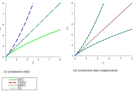
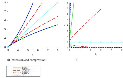
The simplest pattern of loci is given for the incompressible case (υ = ½, figure 5a; see also Literature Review and Treloar, 1975). In this case: J = 1 by definition; the locus for fixed-width extension compression (FWE/C) coincides with that for simple shear (SS); the locus for equibiaxial compression coincides with that for simple extension; the locus for simple compression coincides with that for equibiaxial extension.

Figure 5.a. Loci for simple extension and compression (SE/C), equibiaxial extension and compression (EBE/C) fixed width extension and compression (FWE/C) and simple shear (SS) for

υ

=

.

(ii) (extension and compression)

3 4 5 6 7 8

3 4 5 6 7 8

3 4 5 6 7 8

3 4 5 6 7 8

30

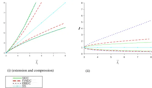
Figure 5.b shows loci for υ = 0.25. A value of 0.25 coincides with: the value predicted (in extension) by the simple structure-based model of Gent & Thomas (1959, 1963) for Poisson’s ratio (ν); the value of the Poisson ratio which Blatz & Ko found for a rubbery foam in SE, EBE and FWE. Also, a value of υ = 0.25 is quite close to: Mott & Roland’s lower limit for ν for normal elastic solids (0.2); the value indicated by the data of Storåkers (1986) for a natural rubber foam (υ ≈ 0.33); the average value of Poisson’s ratio (ν) found by Gent & Thomas for 13 natural rubber latex foams (ν ≈ 0.33) – see also the summary graph in the literature review; the value of ⅓ predicted by the Gibson & Ashby (1982) model.

The projections onto an I1, I2plane of constant J for the loci for SE/C and EBE/C remain

coincident with each other and are on the same curves as they were for the incompressible case; this holds true for all -1 < υ ≤ ½. However, it is clear that for a given value of I1 _the

values of J are very different in simple extension (SE) and equibiaxial extension (EBE).

As expected, Figure 5.b shows that the locus for SS at υ = 0.25 is as it was at υ = 0.5: it remains a straight line of J = 1, I1 I2; as stated above, this holds true for all -1 < υ ≤ ½.

However the locus for FWE/C is no longer coincident with that for SS. Instead, the loci for FWE/C and for SE/C have become rather close inI1, I2, J space.

For a given I₁ and for J > 1 the value of J for the various modes of deformation are in the order: SS (lowest, J = 1), SE/C, FWE/C, EBE/C (highest).

(i) (extension and compression) 3

4 5 6 7 8

3 4 5 6 7 8 0

1 2 3 4 5 6 7 8

3 4 5 6 7 8

J

(ii)

31

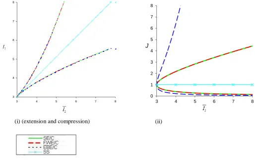
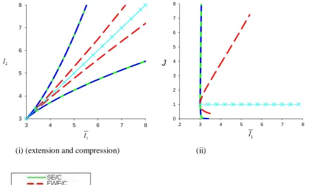
Figure 5.c shows loci for υ = 0 and marks the boundary between ‘normal’ and auxetic behaviour.(But see Mott & Roland, 2013.) As might be expected, the loci for FWE/C and SE/C are now coincident in I1, I2, J space. However, unsurprisingly, the locus for EBE/C

shows considerably greater volume increase (at any given I1) than do the loci for FWE/C and

SE/C.

0 1 2 3 4 5 6 7 8

3 4 5 6 7 8

J

(ii) 3

4 5 6 7 8

3 4 5 6 7 8

.

.

(i) (extension and compression)

32

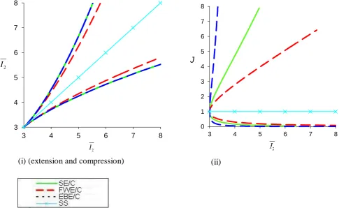
Figure 5.d shows loci for υ = -0.25 and thus gives some insight into auxetic behaviour. The locus of FWE/C on the I₁,I₂ plane has moved back inwards from the locus of SE/C and EBE/C. For a given I₁ and for J > 1 the value of J for the various modes of deformation are now in the order: SS (lowest, J = 1), FWE/C, SE/C, EBE/C (highest). (For J < 1 the order is reversed.) So compared to what was the case for υ = 0.25, FWE/C and SE/C have changed places; this holds true for all -1 < υ < 0.

Except for SS, J changes strongly as I₁varies for each mode of deformation at υ = -0.25.

Figure 5.d (i-ii). Loci for simple extension and compression (SE/C), equibiaxial extension and compression (EBE/C) fixed width extension and compression (FWE/C) and simple shear (SS) for υ = -0.25.

(ii) (i) (extension and compression)

2

I 2

I

0 1 2 3 4 5 6 7 8

3 4 5 6 7 8

J

3 4 5 6 7 8

3 4 5 6 7 8

2

33

Figure 5.e shows loci for υ = -0.5 and thus gives some insight into more auxetic behaviour. The locus of FWE/C on the I1,I2 plane has moved inwards further from the locus of SE/C

and EBE/C.

For EBE/C and SE/C J changes noticeably more strongly with I₁than was the case at

υ = -0.25. 3

4 5 6 7 8

3 4 5 6 7 8

Figure 5.e (i-ii). Loci for simple extension and compression (SE/C), equibiaxial extension and compression (EBE/C) fixed width extension and compression (FWE/C) and simple shear (SS) for

υ

= -

.

34

Figure 5.f shows loci for υ = -0.75 and thus gives some insight into still more auxetic behaviour. The locus of FWE/C on the I₁,I₂ plane is now quite close to the locus of SS. For EBE/C and SE/C the dependence of J on I₁is now so strong that, except at very small values of J, it is difficult to distinguish the loci from a line parallel to the J axis and passing through I₁ = 3.

3 4 5 6 7 8

3 4 5 6 7 8

(i) (extension and compression)

Figure 5.f (i-ii). Loci for simple extension and compression (SE/C), equibiaxial extension and compression (EBE/C) fixed width extension and compression (FWE/C) and simple shear (SS) for

υ

= -

.

(ii) 0

1 2 3 4 5 6 7 8

2 3 4 5 6 7 8

J

1

35

Figure 5.g shows loci for υ = -0.9999 and thus gives some insight into still more extreme auxetic behaviour. The locus of FWE/C on the I1,I2 plane is now essentially coincident with

the locus of SS – qv figure 5.a.

For EBE/C and SE/C the dependence of J on I₁is now so strong that it is virtually

impossible to distinguish the loci from a line parallel to the J axis and passing through I1 =

3. For FWE/C the dependence of J on I1at υ = -0.9999 is somewhat similar to that at υ =

-0.75.

3 4 5 6 7 8

3 4 5 6 7 8

0 1 2 3 4 5 6 7 8

2 3 4 5 6 7 8

J

Figure 5.g (i-ii). Loci for simple extension and compression (SE/C), equibiaxial extension and compression (EBE/C) fixed width extension and compression (FWE/C) and simple shear (SS) for υ = -0.9999.

36

Summary of work on loci in I₁,I₂,Jspace

37

4.2 Generalisation of Blatz & Ko’s approach and behaviour in specific modes of deformation

4.2.1 Generalisation of Blatz & Ko’s approach

As indicated in chapter 2 Blatz & Ko (1962) described an isotropic hyperelastic compressible material by: index. Poisson the is ratio; volume the is n tensor; deformatio Green Cauchy left d neutralise volume the , of invariants principal first two the are and density; energy strain the is : where (4.2.1) 1 2 1 3 1 2 1 3 2 1 2 1 2 2 3 / 2 2 2 1 2 1 3 / 2 1      _   J B I I W J I J C J I J C W                                               

This is a particularisation of the general approach (see Rivlin, 1992 for example) in which the material is described by the dependence of W on I₁ ,I₂ andJ or

J / W I / W I /

W     

 ₁ , ₂ and on I₁ ,I₂ andJ . In equation 4.2.1:

(a) the dependence of ∂W/∂J on I₁ ,I₂ andJ is described via the Poisson index (υ); (b) the Poisson index does not vary with I₁ ,I₂ or J;

(c) W/I₁and W/I₂do not vary with I₁or I₂ - so Blatz & Ko’s equation 4.2.1 can be described as a Mooney-related form of constitutive law.

For Blatz & Ko’s form

(4.2.2c) 2 1 2 1 (4.2.2b) (4.2.2a) 2 1 1 4 3 5 2 2 1 1 3 1 1 3 2 2 2 3 2 1 1         _           _                         J