Multi-Scale Depth from Slope with Weights
Rafael F. V. Saracchini1 [email protected]
Jorge Stolfi1 [email protected]
Helena C. G. Leitão2 [email protected]
Gary A. Atkinson3 [email protected]
Melvyn L. Smith3 [email protected]
1Computer Institute
State University of Campinas Campinas, Brazil
2Computer Institute
Federal Fluminense University Niteroi, Brazil
3Machine Vision Laboratory
University of West England Bristol, UK
Abstract
We describe a robust method to recover the depth coordinate from a normal or slope map of a scene, obtained e.g. through photometric stereo or interferometry. The key feature of our method is the fast solution of the Poisson-like integration equations by a multi-scale iterative technique. The method accepts a weight map that can be used to exclude regions where the slope information is missing or untrusted, and to allow the integration of height maps with linear discontinuities (such as along object silhouettes) which are not recorded in the slope maps. Except for pathological cases, the memory and time costs of our method are typically proportional to the number of pixels N. Tests show that our method is as accurate as the best weighted slope integrators, but substantially more efficient in time and space.
1
Introduction
The integration of a slope map to yield a height (or depth) map is a critical step in ma-chine vision techniques such as shape-from-shading [11,12] and multiple-light photometric stereo [13,28]. Photometric stereo is a promising technology for 3D data capture in many applications, as shown in figure1. It has a number of inherent advantages over other compet-ing techniques,such as laser and stereo triangulation; includcompet-ing lower hardware cost, higher resolution, and simultaneous albedo recovery. A major obstacle to its wider use is the cost and fragility of current slope map integration algorithms — which are the topic of this paper. Abstractly, the goal is to determine an unknown real function Z of some D⊆R2, given its gradient∇Z= (∂Z/∂x,∂Z/∂y). That is, find Z such that ∂Z/∂x=F and∂Z/∂y=G, where F and G are two given real functions. This problem has a differentiable solution if and only if the field(F,G)is curl-free, that is∂F/∂y−∂G/∂x=0 everywhere. Then Z(x,y)
can be expressed as a line integral along any path from a reference point(x0,y0)to(x,y). In practical contexts, however, there are at least three difficulties with this approach. First, the slope functions F and G are generally discretised, i.e. known only at certain slope
c
2010. The copyright of this document resides with its authors. It may be distributed unchanged freely in print or electronic forms.
sampling points p[u,v], which usually form a regular orthogonal grid. Second, the data is usually contaminated with noise arising from unavoidable measurement, quantization, and computation errors. At some points, the expected magnitude of the error may be so high that the slope is essentially unknown; and this may happen over large regions of the do-main D. Third, the height function Z is usually discontinuous. The height field Z(x,y)of a real scene almost always has cliffs—step-like discontinuities along the silhouettes of solid objects. Some slope acquisition technologies, including most photometric stereo methods, will severely underestimate the mean slope across cliffs. Slope values will also be mean-ingless wherever the height itself is poorly defined, e.g. where the scene is highly porous, transparent, or covered with hair. In general, neither the position nor the magnitude of these anomalies can be deduced from the slope maps alone. Because of these complications, several integration methods that have been described in the literature (see section2) are un-suitable for photometric stereo, either for being too sensitive to noise and cliffs, or for being too costly for use with high-resolution maps.
Figure 1: Some applications of slope integration in photometric stereo: 3D face capture [10], security inspections [25], archaeology [14,21], and dermatology [24].
2
Related Work
Most of the previous algorithms for the integration of slope maps can be classified into four broad groups: path integration, Fourier filtering, local iteration, and direct system solving.
Path-integration methods assign a height to one reference pixel p and then compute the
height of every other pixel q by performing a numerical line integral of the gradient field along a path from p to q. This group includes the naive row-by-row integration [29] as well as other methods that choose the paths so as to avoid low-quality or missing data—e.g. by finding an optimum spanning tree and integraling along it, as done by Fraile and Hancock [2,
7]. These methods are generally quite fast, since they require only O(N)operations for an image with N pixels. However, they are very sensitive to noise and discontinuities: if the heights of two adjacent pixels p′,p′′are computed by distinct paths, integration of the noise component of the gradient will result in a spurious height diference between them.
This problem can be alleviated, but not soved, by averaging the integral along many distinct paths between the two pixels [20]. While this approach gets rid of spurious steps due to noise, its cost is prohibitive (proportional to N2.5for an image with N pixels) and its results are still inferior to those of non-path methods described below.
Fourier filtering methods are based on the observation that integrating a function
corre-sponds to dividing each component of the Fourier transform by 2πtimes its frequency. This approach was pioneered by Frankot and Chellapa [8]. In the frequency domain the curl component of the gradient data can be easily filtered out, and other smoothing filters can be applied as well [27]. Fourier techniques can be used also to efficiently solve the unweighted Poisson equation (see below) as done by Georghiades et al. [9].
Through the use of fast Fourier transform algorithms (FFT or DCT), these methods ob-tain the height field for N pixels using only O(N)space and O(N log N)operations. However, this approach does not allow the use of a weight map, because the FFT always gives the same weight to all data samples. As a result, these methods will flatten out any invisible cliffs and deform the surface over a wide area surrounding them.
Local iteration methods reduce the slope integration problem to a system of N equations
whose unknowns are the N heights, and where each equation relates one height value and its neighbours to the given derivatives in that neighbourhood. The equations (whether linear or non-linear) are then solved as in the Gauss-Seidel iterative method: starting with some initial guess, each equation is solved in turn to recompute one height value, assuming the neighbours are fixed, until all the heights appear to stabilise [11,18].
The local equations can be derived in several ways [3,11,22]. However, all these local criteria generally yield some discrete (and possibly non-linear) version of Poisson’s equation
∇2Z=h(x,y). Since each equation refers to a small number of height values, the whole
system uses only O(N)storage. This formulation, unlike path-integration methods, does not generate spurious steps in the presence of noise. Indeed, the solution is theoretically equal to that of the Fourier filtering. The advantage of the iterative formulation, as pointed out by Agrawal et al. in 2006 [3], is that each equation can be tuned to ignore bad data samples and suspected discontinuities, as indicated by a weight map. On the other hand, although each iteration requires only O(N)operations, the number of iterations needed to reduce the error below a specified tolerance is usually proportional to the square of the image’s diameter, that is to N; so the total running time is proportional to N2.
solves a sequence of N×N Poisson systems, where at stage k each height z[u,v]is related to heights z[u±2k,v±2k]. While the use of longer strides substantially improved the conver-gence of the iteration, the speed and accuracy of this method were still quite inferior to those of Fourier-based algorithms.
Direct system solving methods also set up an N×N system of equations from local con-straints, but solve the system by a direct method, such as Gaussian LU or Cholesky factor-ization. (If the equations are non-linear, they must be linearized and the process must be iterated over, as as in the Newton-Raphson method.) This approach is used, in particular, by several of Agrawal’s “Poisson based” methods. [3].
Direct solution methods are generally slower than Fourier methods but much faster than iterative ones. However, their running time grows like O(N1.5), according our tests; and their memory requirements (even with good sparse matrix software) makes them impractical for multi-megapixel slope maps.
3
Weighted multiscale integration
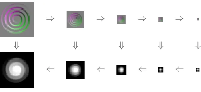
Our multiscale integrator builds the linear equation system for a weighted variant of the discrete Poisson problem, and solves it by the Gauss-Seidel (or Gauss-Jacobi) iterative algo-rithm. Unlike other local iterative methods, it obtains the initial guess by recursively solving a reduced scale version of the problem. Namely, it reduces the given slope maps f,g,w to one half of their original width and height, recursively computes from them a reduced-scale height map z, expands the latter to twice its size, and uses the Gauss-Seidel iteration to ad-just this map accoding to the full-scale slope data. The recursion stops at a level m where the slope maps are so small that the iteration will quickly converges from any initial guess. See figure2.
⇒
⇒
⇒
⇒
⇓
⇓
⇓
⇓
⇓
[image:4.408.45.368.347.495.2]⇐
⇐
⇐
⇐
3.1
The algorithm
The central part of our algorithm is the recursive procedure ComputeHeights below:
ComputeHeights(f,g,w)
1. If f is small enough then 2. z←(0,0, . . . ,0); 3. else
4. f′←ShrinkSlopes(f,w); g′←ShrinkSlopes(g,w); 5. w′←ShrinkWeights(w);
6. z′←ComputeHeights(f′,g′,w′); 7. z←ExpandHeights(z′);
8. A,b←BuildSystem(f,g,w); 9. z←SolveSystem(A,b,z); 10. Return z.
Note that our scheme differs substantially from the “pyramid-based” method of Chen, Wang and Wang [6], since at each scale k we build a Poisson system with only N/4kunknowns,
instead of N.
Inputs: The the slope maps f,g and the weight map w should be three real-valued arrays with the same dimensions. Each sample f[u,v]is assumed to be an average of∂Z/∂x around the slope sampling point p[u,v] = (u+1/2,v+1/2); and similarly for g[u,v]. Each weight w[u,v]should be a non-negative number reflecting the relative trustworthiness of the corre-sponding slope values f[u,v], g[u,v]. The weight w[u,v]should be zero if the corresponding slopes are completely unreliable — in particular, if there may be a cliff crossing the pixel centered at p[u,v]. In that case, the data f[u,v]and g[u,v]will be completely ignored. Our algorithm assumes that w[u,v] =0 also for any pixels theat lie outside the domain D.
Outputs: The algorithm returns an array of height samples z[u,v], nominally taken at height sampling points q[u,v] = (u,v), displaced from the slope sampling points p[u,v]by half a step in each direction. Because of these assumptions, the z array computed by our method will have one more column and one more row than the slope maps.
Building the system: Like other Poisson-based methods [18,26], our algorithm builds in step8a linear equation system with one equation and one unknown for each height value z[u,v]. Each equation states the equality between two estimates of Laplacian L(z) =∇·(∇Z)
at the point q[u,v]: one computed from the unknown heights (the left-hand side), and one from the given slope values (the right-hand side).
The precise nature of the estimates is not critical; our multiscale iterative method can be used with other Laplacian estimators, including non-linear ones. In our implementa-tion [17], we use the equation−L(z)[u,v] =−D(f,g)[u,v], where
−L(z)[u,v] = z[u,v]−w−0 w00
z−0− w+0 w00
z+0− w0−
w00 z0−−
w0+
w00
z0+ (1)
−D(f,g) = w−− w00
f−−+ w−+
w00 f−+−
w+− w00
f+−− w++
w00 f++
+ w−−
w00 g−−+
w+− w00
g+−− w−+
w00 g−+−
w++
w00 g++
and, for all r,s∈ {−,+}={−1,+1},
frs = f[u+r,v+s] grs = g[u+r,v+s] wrs = w[u+r,v+s]
w0s = w+s+w−s wr0 = wr++wr− w00 = w0++w0−+w−0+w+0
z0s = z[u,v+s] zr0 = z[u+r,v]
(3)
Boundary cases: These formulas assume that the weight w[u,v]is 0 if the corresponding point lies outside the domain D. With this convention, equation (3.1) can be used even along the margins of the domain D, or at grid corners q[u,v] that are adjacent to missing slope data. As long as one of the slope samples surrouding a point q[u,v]has nonzero weight, equation is valid and can be used to compute z[u,v]from its neighbours. As a consequence, the algorithm will patch up isolated one- to three-pixel “holes” in the data by integrating around them.
Indeterminate values: On the other hand, when all four slope values surrounding a pixel
are missing the value of z[u,v]is essentially indeterminate. One may exclude those height values from the linear system, and set them to 0,NAN, or any other arbitrary value.
Analysis: To analyse the efficiency of this algorithm, we should consider what the steps do in
the frequency domain. When the slope maps are reduced, the higher-frequency components of the data are lost, while the remaining lower-frequency components have their wavelengths reduced by one half. Therefore, the recursively computed solution z(k+1) to the reduced problem, after being expanded to the original scale, will be mostly correct in the lower frequencies; only the small detail (at the scale of one or two pixels) will be missing. These details will be fixed by the Gauss-Seidel solver after a small number of iterations, largely independent of N. So, the recursive process is fast because each Fourier component of the height map gets computed at the scale where its wavelength is only a few pixels. Therefore, the time spent at scale k will be proportional N/4k; and the total time for all scales will be
(1+1/4+1/42+· · ·1/4m)O(N)<(4/3)O(N) =O(N).
4
Robustness and accuracy
To test the robustness and accuracy of our method, we compared its output with that of representative implementations of the main competing methods.
Data sets: We used the slope datasets and weight maps shown in figure3. The setssbabel,
spdome, andcbrampwere derived from mathematically defined height fields Z(x,y). The
sbabelfield isC1-smooth except at the ends of the ramp, with steep but not vertical walls.
Thespdomefield has a slope discontinuity around the dome’s rim. Thecbrampfield is
C1-smooth along the ramp but has vertical cliffs on three sides. The gradient maps were
obtained by Hann-weighted subsampling of the analytic derivatives, a process that results in some sampling noise at gradient discontinuities, and is completely oblivious to cliffs. In particular, the the cliffs around the top platform ofcbrampare completely invisible in its slope map, and their location is defined only by the zeros in the given weight map. The
psfacedata set is the gradient field of a human face, obtained by photometric stereo [10].
Its binary weight mask, manually created with an image editor, excludes regions where the data is known to be unreliable.
implementations [1], adapted to use our input and output file formats. Methods AS, EM, ME, AT use the weighted Poisson-based approach, with Matlab’s sparse matrix solver; the first three use iterative weight adjustment. However in AS and EM the weight map is internal and is neither accepted not returned by the code. UP is an unweighted Poisson method whose linear system is solved by discrete cosine transfom.
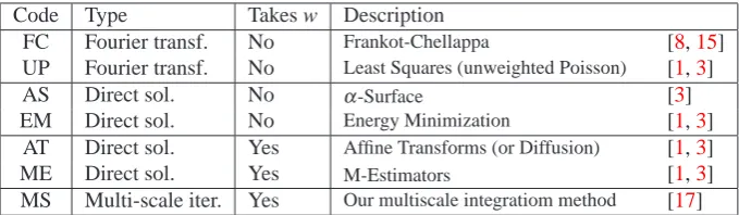
Table 1: Methods used in the accuracy tests.
Code Type Takes w Description
FC Fourier transf. No Frankot-Chellappa [8,15]
UP Fourier transf. No Least Squares (unweighted Poisson) [1,3]
AS Direct sol. No α-Surface [3]
EM Direct sol. No Energy Minimization [1,3]
AT Direct sol. Yes Affine Transforms (or Diffusion) [1,3]
ME Direct sol. Yes M-Estimators [1,3]
MS Multi-scale iter. Yes Our multiscale integratiom method [17]
Reference solutions: Ideally, the accuracy of a slope integrator should be evaluated by
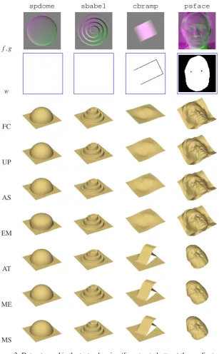
comparing the computed z values with the “true” height field. However, this information is not available for the thepsfacedataset, and its slope data is known to contain substantial localized errors due to highlights and other non-Lambertian features. Even the synthetic data are affected by gradient sampling noise in regions of high curvature. Thus, if we compared the integrated field with the original function Z(x,y)or with laser-range height maps we would not be able to separate the effects of data errors from errors introduced by the integrator. Therefore, we choose to evaluate the accuracy of each method by comparing its output to that of Agrawal’s M-Estimators (ME) method, which appears to be the most accurate and robust of the integrators we tested, and accurately reproduces the true height field of the synthetic maps. In each case we computed the RMS error e between the two integrated height fields, after shifting both to have zero mean; and the relative RMS error e/R, where R is the RMS value of the two height fields. In these computations we considered only the parts of the domain where the weight field w was nonzero.
Results and conclusions: As table 2 and figure3 show, the only methods that obtained usable results in all data sets were Agrawal’s Affine Transforms (AT) and M-Estimators (ME) methods, and our multiscale method (MS). The unweighted methods (FC and UP) and those which do not accept external weight maps (AS and EM) failed completely on the datasets with cliffs and invalid data.
spdome sbabel cbramp psface
f,g
w
FC
UP
AS
EM
AT
ME
[image:8.408.44.352.26.523.2]MS
Figure 3: Datasets used in the tests, showing (from top to bottom) the gradient map
Table 2: Relative RMS errors of each method from the ME reference solution.
spdome sbabel cbramp psface
Meth. e e/R e e/R e e/R e e/R
FC 0.66 1.9% 0.56 2.1% 29.99 120.1% 19.47 98.0%
UP 0.14 0.4% 0.00 0.0% 29.61 107.1% 28.94 114.6%
AS 2.28 6.6% 3.22 12.5% 29.30 107.7% 29.76 106.0%
EM 4.82 13.4% 2.14 8.0% 29.61 107.0% 24.67 108.7%
AT 1.77 5.1% 3.17 12.3% 0.00 0.0% 0.10 0.7%
ME 0.00 0.0% 0.00 0.0% 0.00 0.0% 0.00 0.0%
MS 0.67 1.9% 0.60 2.2% 4.23 13.0% 0.73 3.9%
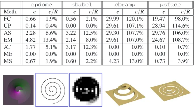
Figure 4: A pathological case for multiscale integration. From left to right: f(0) and w(0)(256×256), w(4)(16×16), and the heights z obtained by ME and by our algorithm with 200 iterations per level.
5
Time and memory
Datasets and methods: To evaluate the efficiency of our method, we measured the
comput-ing time and memory needed for the integration of two square gradient fields,spdomeand
psface, sampled with various grid sizes from 64×64 to 512×512.
We compared our method against two weighted Poisson integrators provided by Agrawal et al. [1], namely the Affine Transforms method (AT) and the weighted Poisson system builder and solver (PC) that is the innermost loop of their M-Estimator, Energy Minimisation, andα-Surface methods. We removed the outermost loop of these last three methods since we are concerned only with the integration problem, not the problem of inferring the weight map. Those are the only methods in the literature that accept a reliability weight map (thus solving the same problem as ours) and are fast enough for practical use.
Results and conclusions: The results of these tests are shown in figure5. The absolute runing times are not directly comparable since our code is in C while the other methods are in Matlab/Octave. However, the plots in figure5 (top) show that the running times scale quite differently: like O(N)for our algorithm (solid line). and apparently like O(N1.5)for the direct Poisson solvers (dashed lines).
Our multiscale integrator also uses less memory than the direct solvers; see figure 5
(bottom). Its memory usage is dominated by the Poisson system’s matrix A which has at most 5N nonzero entriesit uses 60N bytes for A and 5N bytes for the reduced-scale maps. The direct solving methods need to store the matrix A and also Gauss’s triangular factor U (or Cholesky’s R). For these methods, we counted the nonzero entries NAin A and NU in
U , and estimated the memory usage conservativley as 12NA+16NUbytes. We observed that
0.01 0.1 1 10 100 1000
64x64 128x128 256x256 512x512 spdome (sec) AT PC MS 0.01 0.1 1 10 100 1000
64x64 128x128 256x256 512x512 psface (sec) AT PC MS 0.1 1 10 100 1000
64x64 128x128 256x256 512x512 spdome (MB) AT PC MS 0.1 1 10 100 1000
64x64 128x128 256x256 512x512 psface (MB)
[image:10.408.67.342.37.211.2]AT PC MS
Figure 5: Top: Log-log plots of the running time of two direct solving methods (PC,AT) and of our multiscale method (MS), in seconds. Bottom: Log-log plots of memory usage for the system’s matrix A and its U factor (if any), in MBytes.
6
Conclusions
Our weighted multiscale integration algorithm is substantially faster and uses substantially less memory than other methods with comparable accuracy and robustness, both in practice and asymptotically. As fas as we know, ours is the only method that can integrate slope maps of megapixel resolution, with missing data and cliffs of unknown height, within practical memory and time limits. It can be used on its own, with a given weight mask, or as the core of other methods that attempt to deduce the weight mask from the slope data and other clues. Out method can also be adapted to use other estimators for the Laplacian and divergent.
7
Acknowledgments
This work was partially funded by the UWE, by the Brazilian agencies FAPESP (grants 2007/59509-9 and 2007/52015-0), CNPq (grant 301016/92-5 and 550905/07-3), and CAPES (grant 342109-0) and by the UK Research Concil EPSRC (grant EP/E028659/1).
References
[1] A. Agrawal. Matlab/Octave code for robust surface reconstruction from 2d
gra-dient fields. Available from http://www.umiacs.umd.edu/~aagrawal
/software.html. Accessed on 2010-05-01, 2006. See [3].
[3] A. Agrawal, R. Raskar, and R. Chellappa. What is the range of surface reconstructions from a gradient field? In Proc. 9th European Conf. on Computer Vision (ECCV), volume 3951, pages 578–591, 2006.
[4] G. A. Atkinson and E. R. Hancock. Surface reconstruction using polarization and photometric stereo. In Proc. 12th Intl. Conf. on Computer Analysis of Images and Patterns (CAIP), volume 4673, pages 466–473, 2007.
[5] M. Chandraker, S. Agarwal, and D. Kriegman. ShadowCuts: Photometric stereo with shadows. In CVPR07, pages 1–8, 2007.
[6] Y. Chen, H. Wang, and Y. Wang. Pyramid surface reconstruction from normal. In Proc. 3rd IEEE Intl. Conf. on Image and Graphics (ICIG), pages 464–467, 2004.
[7] R. Fraile and E. R. Hancock. Combinatorial surface integration. In Proc. 18th Intl. Conf. on Pattern Recognition (ICPR’06) Volume 1, pages 59–62, 2006.
[8] R. T. Frankot and R. Chellappa. A method for enforcing integrability in shape from shading algorithms. IEEE Trans. Pattern Analysis and Machine Intelligence, 10(4): 439–451, 1988.
[9] A. S. Georghiades, P. N. Belhumeur, and D. J. Kriegman. From few to many: Illu-mination cone models for face recognition under variable lighting and pose. IEEE Transactions on Pattern Analysis and Machine Intelligence, 23:643–660, 2001.
[10] M. F. Hansen, G. A. Atkinson, L. N. Smith, and M. L. Smith. 3d face reconstructions from photometric stereo using near infrared and visible light. Computer Vision and Image Understanding, In Press, 2010. doi: 10.1016/j.cviu.2010.03.001.
[11] B. K. P. Horn. Height and gradient from shading. Intl. Journal of Computer Vision, 5 (1):37–75, 1990.
[12] B. K. P. Horn and Michael J. Brooks. Shape from Shading. MIT Press, Cambridge, Mass., 1989.
[13] B. K. P. Horn, R. J. Woodham, and W. M. Silver. Determining shape and reflectance using multiple images. Technical Report AI Memo 490, MIT Artificial Intelligence Laboratory, 1978.
[14] M. Kampel and R. Sablatnig. 3D puzzling of archeological fragments. In Danijel Skocaj, editor, Proc. of 9th Computer Vision Winter Workshop, pages 31–40, 2004.
[15] P. D. Kovesi. frankotchellappa.m: The Frankot-Chellappa gradient integrator in MATLAB/Octave. Univ. of Western Australia,http://www.csse.uwa.edu
.au/~pk/Research/MatlabFns/Shapelet/, 2000.
[16] H. C. G. Leitão, R. F. V. Saracchini, and J. Stolfi. Matching photometric observation vectors with shadows and variable albedo. In Proc. 21th Brazilian Symp. on Computer Graphics and Image Processing (SIBGRAPI), pages 179–186, 2008.
[18] B. K. P.Horn. Height and gradient from shading. Technical Report AI Memo 1105, Massachusetts Institute of Technology, 1989.
[19] D. Reddy, A. Agrawal, and R. Chellappa. Enforcing integrability by error correction using ℓ1-minimization. In Proc. 2009 IEEE Conf. on Computer Vision and Pattern Recognition, pages 2350–2357, 2009.
[20] A. Robles-Kelly and E. R. Hancock. Surface height recovery from surface normals using manifold embedding. In Proc. Intl. Conf. on Image Processing (ICIP), 2004.
[21] R. F. V. Saracchini, J. Stolfi, and H. C. G. Leitão. Shape reconstruction using a gauge-based photometric stereo method. In Proceedings of CLEI, 2009.
[22] G. D. J. Smith and A. G. Bors. Height estimation from vector fields of surface normals. In Proc. IEEE Intl. Conf. on Digital Signal Processing (DSP), pages 1031–1034, 2002.
[23] J. Sun, M. L. Smith, L. N. Smith, S. Midha, and J. Bamber. Object surface recovery using a multi-light photometric stereo technique for non-Lambertian surfaces subject to shadows and specularities. Image and Vision Computing, 25(7):1050–1057, 2007.
[24] J. Sun, M. L. Smith, L. N. Smith, L. Coutts, R. Dabis, C. Harland, and J. Bamber. Reflectance of human skin using colour photometric stereo - with particular application to pigmented lesion analysis. Skin Research and Technology, 14:173–179, 2008.
[25] J. Sun, M. L. Smith, A. R. Farooq, and L. N. Smith. Concealed object perception and recognition using a photometric stereo strategy. In Proc. 11th Intl. Conf. on Advanced Concepts for Intelligent Vision Systems (ACIVS), volume 5807, pages 445–455, 2009.
[26] D. Terzopoulos. The computation of visible-surface representations. IEEE Transac-tions on Pattern Analysis and Machine Intelligence, 10(4):417–438, 1988.
[27] T. Wei and R. Klette. Height from gradient using surface curvature and area constraints. In Proc. 3rd Indian Conf. on Computer Vision, Graphics and Image Processing, 2002.
[28] R. J. Woodham. Photometric method for determining suface orientation from multiple images. Optical Engineering, 19(1):139–144, 1980.