Enhanced Online Programming for
Industrial Robots
Christian Kohrt
A thesis submitted in partial fulfilment of the requirements of the University of the West of England, Bristol, UK
for the degree of Doctor of Philosophy
This research programme was carried out in collaboration with the University of Applied Sciences Landshut, Landshut, Germany
Abstract
Acknowledgment
I thank my director of studies, Dr. Richard Stamp, and my supervisors, Dr. Antony Pipe and Dr. Janice Kiely at the University of the West of England at Bristol. I also thank my supervisor Dr. Gudrun Schiedermeier at the University of Applied Sciences Landshut.
Dr. Richard Stamp guided me through this work. I have learnt a great deal from him about scientific working and writing. I am glad to have had a director of studies who was willing to take a personal interest in his student.
Dr. Gudrun Schiedermeier made my PhD studies at the University of Applied Sciences Landshut possible. I thank her for her guidance, her constant interest in my PhD studies and for providing the robotics laboratory including its special equipment required for the experiments; without that, I would not have been able to accomplish this work.
Dr. Anthony Pipe gave me his advice, valuable comments and constructive discussions. Dr. Janice Kiely was always available for discussions during my PhD studies.
I also thank the persons at the University of the West of England who offered me the opportunity to study for a PhD within the Faculty of Environment and Technology, and who provided me with the academic support necessary to complete this work successfully. In particular, I thank Matthew Guppy for his advice during the studies.
I am thankful to have had the opportunity to conduct my research at the University of Applied Sciences, Landshut. I am grateful to the former President, Prof. Dr. Erwin Blum, and to the former vice President, Prof. Dr. Helmuth Gesch, to support this work.
I am grateful to BMW AG Munich and Hans-Joachim Neubauer for setting the idea for this work and also to Robtec GmbH for giving me insight to professional robot programming and for their support and experience in the field of robotics.
Finally, I thank my wife, to whom I dedicate this thesis, for her patience, encouragement and support during the probably hardest time of this work.
Contents
Contents
1 INTRODUCTION ... 1
2 LITERATURE SURVEY ... 7
2.1 Industrial Manufacture ... 8
2.1.1 Robot Programming ... 8
2.1.2 Manufacture Assistants ... 11
2.2 Modelling of the Robot ... 12
2.3 Configuration Space Discretization ... 13
2.4 Path and Trajectory Planning ... 14
2.4.1 Graph based Path Planning ... 15
2.4.2 Potential Field Based Path Planning ... 20
2.4.3 Harmonic Functions Based Path Planning ... 22
2.4.4 Neural Network Based Path Planning... 23
2.4.5 Movement Planning ... 24
2.5 World Model ... 24
2.6 Vision and Perception ... 27
2.7 Collision Detection and Avoidance ... 28
2.8 Model Driven Software Development ... 29
2.9 Summary ... 29
3 AIMS ... 32
3.1 Motivation ... 33
3.2 Objectives ... 34
4 EXPERIMENTAL ... 37
5 REQUIREMENTS FOR ADOPTION BY INDUSTRY OF ONLINE PROGRAMMING ... 42
5.1 Industrial Production Environment ... 43
Contents
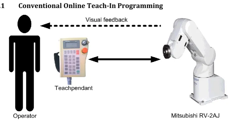
5.2.1 Conventional Online Teach-In Programming ... 47
5.2.2 Offline-Programming Amended by Online Teach-In ... 47
5.3 Identification of Industry Robot Programming Requirements ... 48
5.4 The Proposed Enhanced Online Robot Programming Approach ... 49
5.5 Comparison of Programming Approaches ... 51
5.6 The General Design of the Enhanced Online Programming System ... 52
5.7 Summary ... 55
6 INVESTIGATION INTO A PROBABILISTIC DATA FUSION WORLD MODEL 57 6.1 Cartesian Position Storage ... 59
6.1.1 Index Assignment ... 60
6.1.2 Neighbour and Parent-Child Relations ... 61
6.1.3 Digitalization of the Robot Environment ... 63
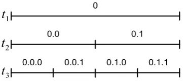
6.2 Robot Joint Position Storage ... 64
6.3 Model Data Storage ... 67
6.4 Data Fusion Framework ... 68
6.5 Vision System... 72
6.5.1 Colour Recognition ... 73
6.5.2 Image Stream Source... 74
6.5.3 Marker Recognition ... 75
6.6 Summary ... 77
7 RESEARCH OF THE ROBOT KINEMATICS MODEL AND THE ROBOT CONTROL CAPABILITIES ... 79
7.1 Mitsubishi RV-2AJ Manipulator Control ... 80
7.1.1 The Built-In Robot Control Modes ... 81
7.1.2 Overview of the built-in Communication Modes ... 82
7.1.3 The Extended Data Link Control Mode ... 83
7.2 Mitsubishi RV-2AJ Kinematics ... 85
7.2.1 The Geometric Solution ... 89
7.2.2 Algebraic Solution ... 92
Contents
7.4 Robotino Kinematics ... 95
7.5 Robot Simulation ... 98
7.6 Summary ... 98
8 INVESTIGATION INTO A TRAJECTORY PLANNING ALGORITHM TO SUPPORT INTUITIVE USE OF THE ROBOT PROGRAMMING SYSTEM ... 99
8.1 Usage Scenarios ... 100
8.2 System Overview ... 103
8.3 Human Machine Interface... 105
8.3.1 Graphical User Interface ... 105
8.3.2 Visual Servo Robot Control ... 111
8.4 Mission Planner ... 112
8.4.1 The General Path Planning Control Loop ... 113
8.4.2 Mission Planning ... 115
8.5 Trajectory Planner ... 118
8.5.1 The General Trajectory Planning Workflow ... 119
8.5.2 Discretization of the Configuration Space ... 121
8.5.3 Reachability Calculation ... 123
8.5.4 The Neural Network Based Roadmap Approach ... 124
8.5.5 The Cell Based Roadmap Approach ... 133
8.5.6 Search within the Roadmap ... 141
8.5.7 Obstacle Types ... 144
8.5.8 Elastic Net Trajectory Generation ... 146
8.6 Robot Program Generation ... 152
8.6.1 Calculating Linear Movements ... 154
8.6.2 Calculating Circular Movements ... 158
8.6.3 Connecting Movement Primitives ... 165
8.7 Summary ... 167
9 RESEARCH OF A SOFTWARE DEVELOPMENT FRAMEWORK FOR COMPLEX SYSTEMS ... 170
9.1 System Modelling ... 172
9.2 Communication Middleware ... 174
Contents
9.4 Toolchain Implementation ... 175
9.5 Connecting Specialized Tools ... 177
9.6 Code Generation Example ... 178
9.7 Summary ... 181
10 SYSTEM IMPLEMENTATION ... 183
10.1 General Workflow ... 185
10.2 Pre-Existing Data Import ... 185
10.3 Mission Preparation ... 185
10.4 Roadmap Generation ... 186
10.5 Path-Planning Application ... 187
10.6 Elastic Net Trajectory Generation ... 188
10.7 Re-planning of the Robot Path ... 190
10.8 Robot Program Generation ... 192
10.9 Robot Programming Duration ... 193
10.10 Summary ... 196
11 DISCUSSION ... 197
12 CONCLUSIONS ... 202
13 FUTURE WORK ... 205
REFERENCES ... 208
A. LIST OF PUBLICATIONS ... 221
B. MATERIALS & EQUIPMENT ... 225
C. ROBOT CONTROL ... 229
D. DENAVIT-HARTENBERG-PARAMETER ... 233
Contents
G. NODE MOVEMENT CALCULATION ... 246
H. PLUGIN MANAGER ... 249
I. SAMPLE SOURCE CODE ... 254
I.1 Message Service ... 254
I.2 Robot Kinematics ... 261
Forward Calculation ... 261
Inverse Calculation ... 262
Common Transformation Equation ... 263
I.3 Program Export ... 264
I.4 Linear Octree and Trajectory Planning ... 265
I. Glossary
I.
Glossary
Configuration space A robot with degrees of freedom is usually a manifold of dimension . This manifold is called the configuration space of the robot, and is considered as a state-space.
Kinematics The study of the motion of bodies without reference to mass or force.
Manufacture assistant Manufacture assistants are clever systems, which help the worker to accomplish their task.
Mission A mission defines a path-planning task with application information and locations.
Octree An octree is a tree data structure in which each internal node has up to eight children. Octrees are most often used to
partition a three dimensional space by recursively subdividing it into eight octants.
Online programming Programming of robots by the help of the teachpendant or other robot control devices with the need of the real robot. Offline programming Programming of robots by the help of a simulation system
without the need of the real robot.
Quadtree A quadtree is a tree data structure in which each internal node has up to four children. Quadtrees are most often used for partitioning by recursively subdividing it into four quadrants. Trajectory The line or curve described by an object moving through
space.
II. List of Abbreviations
II.
List of Abbreviations
Acronym Definition
AD* Anytime Dynamic A* BSP Binary Space Partitioning CAD Computer-Aided Design
CASE Computer-Aided Software Engineering COM Component Object Model
CORBA Common Object Request Broker Architecture DDE Dynamic Data Exchange
DH Denavit Hartenberg DLL Dynamic Link Library DSP digital signal processor DXF Drawing Exchange Format EMF Eclipse Modelling Framework EN Elastic Net
ES Evolution Strategy
FPGA Field Programmable Gate Array GPP General purpose processor GUI Graphical User Interface HMI Human Machine Interface
HSV Hue, Saturation, and Value Colour Space ICE Internet Communication Engine
IP Internet Protocol JET Java Emitter Template JNI Java Native Interface JVM Java Virtual Machine LED Light Emitting Diode MDA Model Driven Architecture MDG Model Driven Generation
NARC New Architecture Robot Controller ODE Open Dynamics Engine
OMG Object Management Group PC Personal Computer
PLC Programmable Logic Controller RBF Radial Basis Function
II. List of Abbreviations
RGB Red, Green, and Blue Colour Space ROOM Real Time Object Oriented Modelling SMA Simple Moving Average
SWT Standard Widget Toolkit TCP Transmission Control Protocol TCP Tool Centre Point
TD Temporal Difference
TSP Traveling Salesman Problem UDP User Datagram Protocol
UK United Kingdom
III. List of Figures
III.
List of Figures
Figure 1: Illustration of the visibility graph (by author). ... 16
Figure 2: Cell decomposition graph (by author). ... 16
Figure 3: Cell decomposition with black obstacles and free space (by author). ... 17
Figure 4: A Voronoi diagram with regions, where each region consists of all points that are closer to one site than to any other (by author). ... 18
Figure 5: Potential field method. ... 21
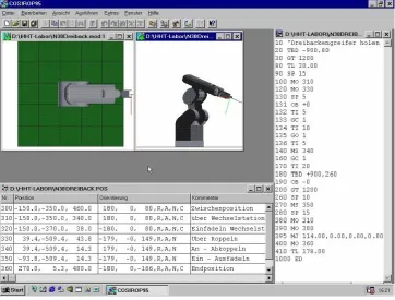
Figure 6: The Cosirop robot programming software. ... 39
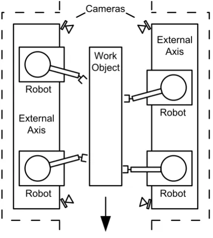
Figure 7: The experimental system. ... 40
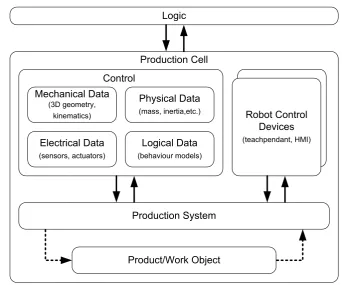
Figure 8: Typical production cell. ... 44
Figure 9: Schematic view of a production cell. ... 45
Figure 10: Robot program structure. ... 46
Figure 11: Production cell life cycle. ... 46
Figure 12: Online teach-in programming. ... 47
Figure 13: Offline-programming amended by online teaching... 47
Figure 14: The enhanced online robot programming approach. ... 49
Figure 15: Overview of the enhanced online programming system. ... 53
Figure 16: Path planning system: a logical view. ... 54
Figure 17: System overview of parts and devices. ... 55
Figure 18: The logical view of the path planning system with the highlighted flow of sensor information. ... 58
Figure 19: A linear octree with two subdivisions. ... 60
Figure 20: Octree data structure representation. ... 61
Figure 21: Four neighbours. ... 62
Figure 22: Eight neighbours. ... 62
Figure 23: The problem with eight neighbours. ... 62
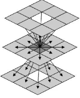
Figure 24: Spatial space neighbour relationship of an octree cell, shown by the arrows. ... 63
Figure 25: The robot environment and relation of world and octree representation. ... 63
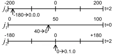
Figure 26: Example robot. ... 64
Figure 27: General joint angle binary tree for a joint 𝑗 with depth 𝑡=3. ... 65
III. List of Figures
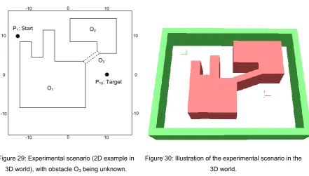
Figure 29: Experimental scenario (2D example in 3D world), with obstacle O3 being
unknown. ... 68
Figure 30: Illustration of the experimental scenario in the 3D world. ... 68
Figure 31:Data sources of the information fusion system. ... 69
Figure 32: Sensor fusion architecture. ... 69
Figure 33: Sensor values derived from real sensors. ... 71
Figure 34: Fused sensor data. ... 71
Figure 35: Image stream processing chain. ... 73
Figure 36: The HSV colour space. ... 74
Figure 37: Colour calibration process. ... 74
Figure 38: Simulink image acquisition block and colour conversion. ... 75
Figure 39: Image stream processing chain. ... 75
Figure 40: Image stream segmentation. ... 76
Figure 41: Blob analysis block. ... 76
Figure 42: Blob analysis block. ... 77
Figure 43: Blob analysis block. ... 77
Figure 44: Schematic representation of forward and inverse kinematics ... 86
Figure 45: Revolute (left) and prismatic (right) joints ... 86
Figure 46: Mitsubishi RV-2AJ joints (from Mitsubishi documentation). ... 87
Figure 47: Mitsubishi RV-2AJ dimensions ... 87
Figure 48: Robot coordinate systems. ... 88
Figure 49: Law of cosine... 89
Figure 50: Geometric inverse calculation for joint 1 ... 89
Figure 51: Geometric inverse calculation for joint 2 and 3 ... 90
Figure 52: Dubins airplane model. ... 93
Figure 53: Industrial manipulator ‘free flying’ model. ... 94
Figure 54: A Robotino robot from the company Festo. ... 95
Figure 55: Local coordinate axes of the Robotino robot... 95
Figure 56: Kinematics of a car like robot. ... 96
Figure 57: Robotino calculations. ... 96
Figure 58: The use cases of the support system. ... 101
III. List of Figures
Figure 62: Graphical-User-Interface controller Finite-State-Machine. ... 109
Figure 63: The dynamic toolbar. ... 110
Figure 64: The dynamic toolbar. ... 111
Figure 65: Visual servo control application. ... 112
Figure 66: The Mission and path planning control loop. ... 114
Figure 67: Logical view of the support system. ... 115
Figure 68: Path length information exchange. ... 115
Figure 69: Definition of the roadmap elements. A1 and A2 set the start and end location of the application path. ... 116
Figure 70: Illustration of possible path connecting three application path for mission task planning. ... 117
Figure 71: Graph of a discretized configuration space. ... 122
Figure 72: Workspace approximation of the obstacles and the free space with robot configuration locations. ... 126
Figure 73: Forces on the safe and unsafe nodes for random inputs, marked as crosses. ... 127
Figure 74: Error-based safe node addition. ... 128
Figure 75: Error-based safe node addition. ... 128
Figure 76: Unsafe nodes on the boundary... 129
Figure 77: Error-based safe node addition. ... 129
Figure 78: Error-based safe node addition. ... 129
Figure 79: Scene-based unsafe node addition. ... 130
Figure 80: Scene-based unsafe node addition. ... 130
Figure 81: Scene-based unsafe node addition. ... 130
Figure 82: Scene based safe node addition. ... 130
Figure 83: Workspace approximation of the obstacles and the free space. ... 131
Figure 84: Simplification of a complex roadmap. ... 131
Figure 85: The shrinking forces. ... 132
Figure 86: Voronoi approximation in a two-dimensional uniform grid. ... 135
Figure 87: Level 1, edge length: 21=2. ... 137
Figure 88: Level 2, edge length: 22=4. ... 137
Figure 89: Level 3, edge length: 23=8. ... 137
Figure 90: Level 4, edge length: 24=16. ... 137
Figure 91: Level 5, edge length: 25=32. ... 137
III. List of Figures
Figure 93: Defined distance influence on Voronoi path generation. ... 140
Figure 94: Roadmap elements. ... 141
Figure 95: Obstacle synchronization. ... 144
Figure 96: Correlation between e and the radius r in a circle (2D). ... 147
Figure 97: Correlation between e and the radius r in a polygon (2D)... 147
Figure 98: Installed forces. ... 148
Figure 99: Angles of the rotational force. ... 149
Figure 100: Path with ta,min = 0. ... 151
Figure 101: Path with ta,min > 0. ... 152
Figure 102: Linear Movement corridor (highlighted in red) calculation with three points P0-2. ... 155
Figure 103: New node not touching the corridor. ... 157
Figure 104: Planes calculated from connected nodes. ... 159
Figure 105: Calculation of the allowed corridor in two dimensions. ... 160
Figure 106: Nodes in a circular segment... 161
Figure 107: Final point calculation. ... 164
Figure 108: Connecting two linear movement primitives... 166
Figure 109: Connecting a linear and a circular Movement. ... 167
Figure 110: Connecting a circular and a linear movement. ... 167
Figure 111: Connecting two circular movements. ... 167
Figure 112: Communication overview: Message passing from component A to component C (dashed arrow). ... 173
Figure 113: Code generation workflow. ... 175
Figure 114: Toolchain implementation. ... 176
Figure 115: Execution environment. ... 177
Figure 116: Node. ... 177
Figure 117: Actor deployment. ... 177
Figure 118: Plugin manager communication. ... 178
Figure 119: Component connections. ... 179
Figure 120: Component interfaces. ... 180
Figure 121: Interface definition. ... 180
III. List of Figures
Figure 125: Roadmap of the scenario (without obstacle O3). ... 187
Figure 126: Roadmap corridor including configuration space positions. ... 188
Figure 127: Trajectory through the roadmap without obstacle O3. ... 189
Figure 128: Elastic net trajectory generation. ... 190
Figure 129: Adding collision indication positions (part of obstacle O3). ... 191
Figure 130: New re-planned path. ... 191
Figure 131: Experimental scenario. ... 192
Figure 132: Automatically planned path. ... 192
Figure 133: Manually planned path. ... 192
Figure 134: Devices overview. ... 225
Figure 135: The Robot manipulator Mitsubishi RV-2AJ. ... 226
Figure 136: CR1 Controller. ... 227
Figure 137: A Robotino robot from the company Festo. ... 228
Figure 138: Constructed coordinate systems. ... 233
Figure 139: Actor with ports. ... 236
Figure 140: Communication overview. ... 238
Figure 141: Running loop of a thread. ... 238
Figure 142: Event scheduling. ... 239
Figure 143: Thread priorities. ... 240
Figure 144: Interrupt handling. ... 241
Figure 145: The Kohonen Map. ... 244
Figure 146: Vectors of movement... 246
IV. List of Tables
IV.
List of Tables
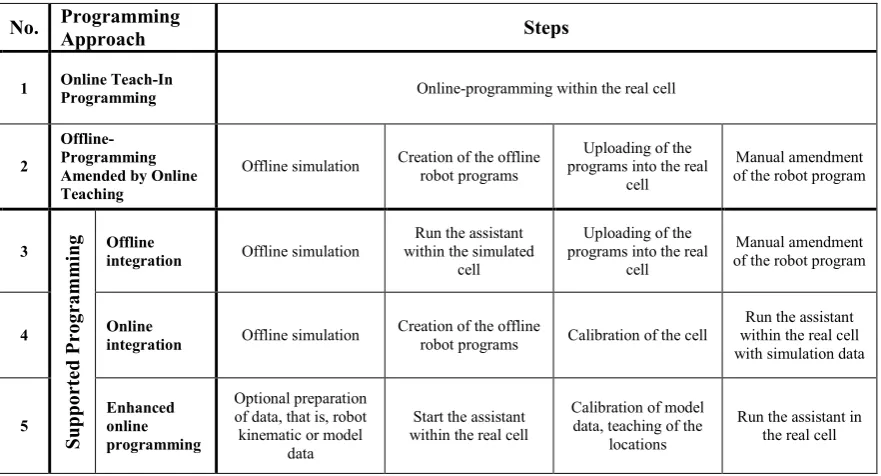
Table 1: The robot programming scenarios. ... 51
Table 2: Comparison of scenarios. ... 52
Table 3: Status of sent commands. ... 82
Table 4: Built-in robot communication modes. ... 83
Table 5: Use cases. ... 83
Table 6: DH-parameters (see also Appendix C). ... 88
Table 7: Path combinations. ... 117
Table 8: Optimal discretization compared to uniform discretization. ... 123
Table 9: Object type definition. ... 145
Table 10: Parameter values. ... 151
Table 11: Path planning execution times. ... 194
Table 12: Comparison of the online programming times. ... 194
Table 13: Comparison of the overall programming times. ... 195
Table 14: Controller communication mode set up. ... 230
Table 15: Controller communication mode set up (continued). ... 231
Table 16: Receive command pattern. ... 232
Table 17: Message parameters. ... 242
Table 18: Mapping of Java data types to native types. ... 250
Table 19: Data types... 252
V. List of Listings
V. List of Listings
1 Introduction
Automated production is essential for industries, including the automotive, electronics, plastics and metal products industries. Automation can be realized by the introduction of industrial robots, which are efficient in terms of speed, flexibility and reliability. At the end of 2010, the worldwide stock of operational industrial robots numbered between 1,030,000 and 1,305,000 units. In 2010, the worldwide market value for robot systems was estimated to be US$5.7 billion (International Federation of Robotics, 2011). The use of robots and automation levels in the industrial sector is expected to continue to grow in future, and will be driven by the on-going need for enhanced productivity. Manufacturing industries continue to be faced with shortened product life cycles, increasing dynamics of innovation, and continuing diversification of their product ranges. Simultaneously, they have to lower the costs per item and the costs of hiring skilled workers. The dynamic requirement profile of production must be addressed in order to ensure compliance with high quality standards as well as time and cost efficiency. Industrial robots are capable of meeting the emerging needs with regards to flexibility and productivity, but the use of these robots remains difficult, time consuming and expensive. There are particularly high requirements in terms of capable robot programming and control technologies. Industries are strongly motivated to improve efficiency and effectiveness of robot programming and control. Production engineering and automation have been developed to an advanced level, and further improvements may be reached using new approaches to the programming of robots. Therefore, the vision of the industry is to realize a completely automated production process without any manual intervention from the product planning stage to the manufactured product. This vision has not been achieved, and even under ideal conditions of production machines, trajectory planning remains difficult. With regard to errors that result from unknowns and falsehoods in the environment, realizing this vision becomes even more unlikely. Robot programming for a specific application may require months, while the cycle time of the application is executed in only a few minutes or hours. Therefore, robotic automation requires that significant investments be made before commencing production.
1 Introduction
production system be put offline and out of production for significant periods of time while the data are manipulated, e.g. upload of or programming of robot programs. This leads to production downtimes and financial loses. It also places a lot of pressure on the operators, which may have an impact on the quality of the created programs. Once the programs are created, it is difficult to make amendments. Nevertheless, conventional online programming is widely used because of its intuitiveness and low initial cost. Advances in online programming simplify the control of the robots, such as Master-Slave programming and demonstrational programming (Demiris and Billard, 2007), but have not yet led to crucial improvements.
1 Introduction
Investigations have been carried out with the aim being to optimize the robot-programming methodology for industrial high-volume and small-batch manufacturing. To address this aim, two key aspects have been identified that are different but related. First, the reduction of financial investments required that an analysis be made of the current robot programming approaches in order to explore all possible cost reduction options. Because production cost is measured in terms of the product cost, the production volume is an important feature that highlights the difference in the requirements for small-batch and high-volume production. In particular, in the area of small-batch production, the investments required for offline programming are prohibitive, and attention has been turned to developing approaches to online robot programming. High-volume production would also benefit from a change to the online robot programming approach, given that production downtimes are within the current range, and that the functionality of the current offline approach is still supported. A new online robot programming approach has been analysed, with the focus being on the fulfilment of requirements for both production volumes. This has required significant investigations into existing approaches to robot programming, including assisted interaction with the operator to help less experienced operators use this system. An enhanced online robot programming support system has been adopted for this task.
As the second key aspect, online robot programming is very demanding for a requirements-driven trajectory-planning algorithm. This also includes the ability to handle inaccurate information (which may be obtained by sensors) and the environment, as well as pre-existing information. Research has been undertaken to develop a trajectory-planning algorithm and to fuse inaccurate information into an in-memory occupancy grid to represent the production environment. It is understood that the development of large software systems requires a modern software development approach to integrate the entire system that consist of robot control devices, sensors and software components. Research has been carried out to implement a model-driven code generation toolchain.
1 Introduction
throughout this study, which enables the execution of forward and inverse calculations between the robot coordinate system and the world coordinate system. Robot control and modelling are illustrated in Section 5.7. The environment in which the robot operates is stored in a so-called world model, which is an in-memory occupancy grid. Information, such as sensor data and pre-existing models, is fused into the grid to obtain coherent data. The world model and information fusion are illustrated in Chapter 6. Based on robot control and the in-memory occupancy grid, a trajectory-planning algorithm that supports the chosen robot programming approach has been introduced. It also includes path finding, trajectory generation and automated robot program creation that is ready to be uploaded to the real system. The results are stated in Chapter 7. The implementation of the system requires the incorporation of many software and hardware components. A modern software development toolchain has been analysed and implemented to support the development of the enhanced online robot programming support system. Chapter 9 addresses the development toolchain.
Chapter 2 presents a review of the whole research activity covered in this investigation, and it helps to collate important results that address the original aims of the study. The conclusions made are itemised in Chapter 12. Sample source code is presented in Appendix I. The investigation has highlighted particular aspects, many of which were unknown at the beginning of the research described herein, and which could themselves form the basis for additional studies. These are stated in Chapter 13.
1 Introduction
The result of this work leads to an enhanced online robot programming system for robot arms. The proposed system will be a novel, rapid, convenient and flexible method to program industrial robots. Programming within the real environment becomes possible and will decrease offline programming time and render offline simulation systems unnecessary when physical production parts and fixtures are to hand either as real objects or as Computer-Aided Design (CAD) data.
2 Literature Survey
2.1 Industrial Manufacture
Based on the product lifetime and production volume, Hägele et al. (2001) classifies industrial manufacture into conventional, pre-configured, decentralized and assisted manufacturing.
Conventional manufacturing lines can be effectively employed when the product lifetime and the production volume are known beforehand. The degree of automation is based on the technological feasibility and cost of each operation.
Pre-configured robot work cells produced in medium numbers at low cost for standard manufacturing processes such as welding, painting and palletising may even be cost-effective when operated below full capacity (Westkämper et al., 1999).
Modern decentralized paradigms restructure the production into a network of configurable working cells, which are connected such that they achieve flexibility in terms of changing products. These production cells are often called ‘holonic’ or ‘bionic’ manufacturing systems (Westkämper et al., 1999).
The greatest flexibility is required in assisted manufacturing co-operating with the worker in handling, transporting, machining and assembly tasks (Hägele et al., 2002, Kristensen et al., 2001, Kristensen et al., 2002, Prassler et al., 2002, Stopp et al., 2002, Thiemermann, 2005, Wösch et al., 2002).
Motion planning is required for any of the above-mentioned types of manufacturing. Assisted manufacturing is based on reactive motion planning, whereas conventional, pre-configured and decentralized manufacturing processes are often based on fixed robot programs, and are further explained in Subsection 2.1.1. The limitation of fixed robot programs is reached when the task execution requires a level of perception, dexterity and decision making which cannot be met technically in a cost effective or robust way. To achieve better productivity, assisted manufacturing relies on the co-operation between the robot and the operator. These robots can be considered to be manufacturing assistants, and are further described in Subsection 2.1.2.
2.1.1 Robot Programming
2 Literature Survey
engineer in the office. It has its strength in the programming of complex systems, and it has been proven to be more efficient and cost-effective for production with large volumes.
Pan et al. (2010) reviews modern robot programming approaches and summarizes sensor-assisted online programming and offline programming approaches. Advancements in online programming have led to a simplification of the control of the robots, such as Master-Slave programming and demonstrational programming, but they have not yet led to any significant improvements. Offline programming reduces the production downtimes by creating the robot programs beforehand with a simulation system (Kain et al., 2008, Maletzki et al., 2008, Pan et al., 2010). Nevertheless, the calibration phase and the offline programming phase are still expensive, and result in significant programming effort, large capital investment and long delivery times (Pan et al., 2010).
Online Programming
2 Literature Survey
Offline Programming
High-volume manufacture utilises offline programming to simulate and generate robot programs with specialized simulation software. The software engineer evaluates the reachability, fine-tunes properties of robot movements, and handles the process-related information before generating a program that can be downloaded to the robot. The actual robot is not required for programming, minimizing the production downtime. Usually, robot programs are developed at the beginning of the product development and production cycle. However, a simulation and programming phase executed by skilled engineers is time consuming and requires specialized and expensive simulation software. Thus, small- and medium-volume manufacture does not benefit from this technology (Pan et al., 2010), whereas large companies, for example BMW AG in the automotive industry, apply offline programming as a standard process. High volume production justifies the costly simulation and programming phase in order to assure high quality production.
Offline programming incorporates models of the work pieces, the robots and the environment. While the robot model is usually delivered by the manufacturer, the work pieces and the environment have to be created manually or, for example, with laser scanning (Bi and Sherman, 2007).
Successively, application locations have to be created in a manual or automatic fashion. The offline programming tools often provide functions that are used to extract features, e.g. edges and corners, and which can be utilized to define the required robot application task. Additional aspects related to the application type, e.g. equipment control, have to be considered in order to produce the robot programs. It becomes evident that the software engineer also requires skills in the specific application type to produce high-quality robot programs. The approach proposed by Pires et al. (2004) attempts to extract robot motion information from the models automatically.
2 Literature Survey
The entire production cycle, or parts of it, can be simulated after robot program creation to verify the production process without the physical production system (Heim, 1999). Successively, the robot program can be uploaded and executed within the real production environment. Extensions have been developed, for example by Wenrui and Kampker (1999), to enhance the simulation and offline programming process. In practice, inaccuracies and errors resulting from unknowns and falsehoods in the environment have to be altered manually using the real production system.
2.1.2 Manufacture Assistants
Hägele et al. (2002) describes manufacture assistants as clever systems which help the worker to accomplish their task. However, high-volume manufacturing is presently fully automated, and human-robot interaction is not always required. The high level of automation is attained through the robot-programming task, which is executed once during installation of the production cell. Thus, assisted robot-programming produces a robot program and is distinguished from manufacture assistants. Helms (2002) proposes a ‘human centred automation’ to improve the usability of robots, with the aim being to combine the sensory skill, the knowledge and the skilfulness of the worker with the advantages of the robot, e.g. strength, endurance, speed and accuracy. Manufacturing assistants represent a generalization of industrial robots characterized by their advanced level of interaction. Nevertheless, the human-machine interface and the underlying technology realizing the assistance functionality also play an important role.
The human-machine co-operation has been addressed by numerous researchers, and is viewed as a prime research topic by the robotics community (EURON, 2012). Haegele et al. (2001) also state the typical requirements for the human-machine interface. The human and the robot assistant should co-operate and safely interact, even in complex situations. This implies that the assistant understands the human intent through natural speech, haptic or graphical interfaces. In addition, effective cooperation depends on the recognition and perception of typical production environments, as well as on the understanding of tasks within their own contexts. Effective assistance requires the technical intelligence of the robot as well as the knowledge and skill transfer between the human and the robot.
2 Literature Survey
approaching humans, and presenting objects have to be performed. In the more difficult case of physical contact with the human, typical skills would comprise compliant motion, anthropomorphic grasping and manipulation. A suitable safety concept has to account for the integrity of the system just as it must account for the integrity of its surroundings. External events affecting the proper function of the system and internal error conditions have to be identified beforehand and classified according to their inherent risk factors.
2.2 Modelling of the Robot
The robot manipulator is an essential tool for the development of automated manufacturing. A robot manipulator, also known as robot-arm, is a non-linear system with rotatory joints (Craig, 2003). The motion equations of the robots are coupled, non-linear high-order differential equations, and the expenditure required for their evaluation is generally very high. Either procedures for the evaluation of the motion equations work numerically, or the motion equations are determined in symbolic form. An overview is given by Schiehlen (1990), Paul (1981), Spong et al. (2004) and Kucuk and Bingul (2006). The motion equations of robots may always be produced in closed form, but lead to a high complexity of the equations. Equations in symbolic form are usually much more efficient in the evaluation than the purely numeric procedures, because many simplifications can be employed (Craig, 2003, Fisette and Samin, 1993, Vukobratovic and Kircanski, 1982, Westmacott, 1989).
The Robotics Toolbox for Matlab (Corke, 1996) allows the user to create and manipulate fundamental data types with ease, such as homogeneous transformations, quaternion and trajectories. Functions provided for arbitrary serial-link manipulators include forward and inverse kinematics, and forward and inverse dynamics.
In most cases, the manipulator has to be controlled in the workspace, which is defined by external world coordinates and not in the configuration space, which is defined by internal joint coordinates. Therefore, a transformation between world and configuration space is required (Craig, 2003, Lenz and Pipe, 2003, Maël, 1996, Russell and Norvig, 2002).
2 Literature Survey
The inverse kinematics problem involves finding joint coordinates so that a desired world coordinate is reached. Calculating the inverse kinematics is generally hard, especially for robots with many degrees of freedom. This problem is ill posed because the solution does not have to be unique. In particular, considering an unreachable target, no solution exists at all (Russell and Norvig, 2002).
The kinematics of a robot may also be seen as a non-linear system, which can be approximated by mapping the input space to an output space of a function. Neural networks have the ability to learn such mappings, and they are therefore called ‘function approximators’. A general example with a Continuous Self-Organizing Map is given by Aupetit (2000). Features of neural networks are utilized to learn the kinematics of a robot, which is an open- or closed-loop kinematic chain, and is not often precisely known. Maël (1996) proposes a hierarchical network for visual servo coordination which is based on the publication of Ritter et al. (1992). The hierarchical approach allows the learning of geometric models of realistic robots with six or more axes. The network consists of several one-dimensional sub networks which learn the coordinate transform and rotation axis for each joint below the visual error. A dynamically-sized radial basis function Neural Network was developed by Lenz and Pipe (2003) to control a six-axis Puma 500 robot on a slow 16-bit microcontroller. Following Ge (2004), given a nonlinear robot system, model-based control is superior to non-model-model-based control. On the other hand, for complex nonlinear systems, it is more difficult to obtain a realistic model than to design a working control system in reality.
2.3 Configuration Space Discretization
2 Literature Survey
Thus, the path-planning algorithm does not need to take care of the configuration space of the robot. This is realized by ego-kinematic transformations. Because the kinematic constraints are embedded in the ego-kinematic transformation, the admissible paths are mapped onto straight lines in the transformed space, and each point of the ego-kinematic space may be reached by a straight-line motion of 'free-flying behaviour'.
The state space of the robot configuration space is often infinite. Sampling-based planning algorithms may consider a small number of samples to reduce the running time (LaValle, 2006). Therefore, path planners often use sampling strategies that are based on the specific path planning problem and environment. Known strategies are random and deterministic sampling schemes (LaValle, 2006). Random sampling schemes take samples from the configuration space of the robot in a uniform manner; every state of the configuration space must have an equal opportunity to appear in the sample. Deterministic sampling schemes are pre-defined sampling techniques (LaValle and Kuffner, 2000). They have the advantages of classical grid search approaches and a good uniform coverage of the configuration space, but require long processing times (Branicky et al., 2001, Lavalle
et al., 2000, Lindemann and LaValle, 2004). Reif and Wang developed (2000) an algorithm with non-uniform discretisation for motion planning, where the discretization is greater in regions that are farther from all obstacles.
2.4 Path and Trajectory Planning
Trajectory planning is a fundamental problem, and significant research has been conducted over the past few decades, either in static or in dynamic environments, for example in the process of spray painting (Chen et al., 2008). Trajectory planning includes the generation of a trajectory from the start to the target position, giving consideration to objectives, such as minimizing path distance or motion time, and avoiding obstacles in the environment and satisfying the robot kinematics. Motion planning is usually decomposed into path planning and trajectory tracking. The former generates a nominal trajectory, whereas the latter tracks that trajectory.
2 Literature Survey
Therefore, path-planning algorithms often try to find an approximated solution to reduce computation time (LaValle, 2006). For example, roadmap methods (Geraerts and Overmars, 2002) do not compute the whole configuration space, but try to generate a roadmap of suitable configurations. Apart from roadmap-based techniques, the potential field approach (Koren and Borenstein, 1991, Warren, 1989) and cell-based method (Kitamura et al., 1995, Ranganathan and Koenig, 2004) are two popular path planning approaches.
Path planning often includes searching the shortest path within a given graph. This can be accomplished with shortest-path search algorithms like the Dijkstra, A* or D* (Goto et al., Likhachev et al., 2005, Xiang and Daoxiong, 2011). The A* algorithm is one of the most important algorithms because its implemented heuristic enhances the search algorithm by directing the search to the target node.
2.4.1 Graph based Path Planning
Graph based approaches are also known as skeleton (Yang and Hong, 2007) or roadmap (Bhattacharya and Gavrilova, 2008) approaches. A free space, such as the set of feasible motions, is mapped onto a network of one-dimensional lines. The visibility (Yang and Hong, 2007) and cell decomposition graph (Lingelbach, 2004), Voronoi diagram (Bhattacharya and Gavrilova, 2008) and probabilistic roadmap (Kazemi and Mehrandezh, 2004b) are frequently-used skeletons, and are presented in the following subsections. Visibility Graph
2 Literature Survey
Obstacle
Start
Target
[image:38.595.253.417.74.289.2]Obstacle
Figure 1: Illustration of the visibility graph (by author).
Cell Decomposition Graph
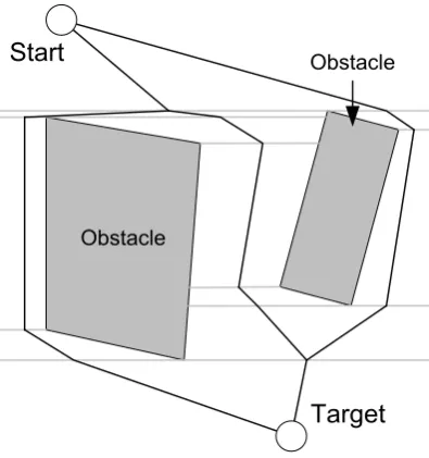
The cell decomposition graph subdivides a given free space into cells. One example of such subdivision is illustrated in Figure 2. The world model, which is the in-memory model of the surrounding, is delimited to a rectangle. For each edge of the obstacles, a horizontal line is included. The bisecting of each line is a point of the graph, and therefore, the horizontal clearance to obstacles is maximized. Extension to a three-dimensional space is difficult and the path obtained in this way is long.
Obstacle
Start
Target
Obstacle
[image:38.595.235.433.490.701.2]2 Literature Survey
Cell decomposition methods generally divide the robot’s free space into cells. The connectivity graph is built by connecting adjacent cells. A channel leading from the start to the target configuration through the graph may then be computed. A path may be chosen leading through the midpoints of the intersections of two successive cells. Examples of grid-based approaches are cell decomposition methods, which convert the configuration space of the robot in discrete cells. The cell division may be either objectdependent or -independent. Both cases are shown in Figure 3. A path is required to connect the start and the target node with a sequence of adjacent cells, which can be computed using a shortest-path search algorithm.
Figure 3: Cell decomposition with black obstacles and free space (by author).
Voronoi Diagrams
2 Literature Survey
Figure 4: A Voronoi diagram with regions, where each region consists of all points that are closer to one site than to any other (by author).
Voronoi diagrams have been shown to be powerful tools in solving seemingly unrelated computational problems, and therefore have increasingly attracted the attention of computer scientists in the last few years. Efficient and reasonably simple techniques have been developed for the computer construction and representation of Voronoi diagrams.
Voronoi-based path planning methods have been studied in literature (Bhattacharya and Gavrilova, 2008, Fortune, 1986, Hoff et al., 2000, Hoff et al., 1999, Kim et al., 2009, Vleugels et al., 1993). The basic properties of a Voronoi diagram are treated by Aurenhammer (1991), who also recommended the publications of Preparata and Shamos (1985) and Edelsbrunner (1987). Hoff et al. (1999) presented a computational algorithm for generalized Voronoi diagrams, and did a survey of existing Voronoi computation algorithms for two and higher dimensions. The presented Voronoi computations are the divide-and-conquer algorithm (Shamos and Hoey, 1975) and the sweep line algorithm (Fortune, 1986). Numerically robust algorithms for constructing Voronoi diagrams have also been proposed in literature (Ingaki et al., 1992, Sugihara and Iri, 1994). Higher-order Voronoi diagram computations have been summarized by Okabe et al. (2008) based on incremental and conquer techniques. The set of algorithms includes divide-and-conquer algorithms for polygons (Lee, 1982, Martin, 1998), an incremental algorithm for polyhedra (Milenkovic, 1993), and three-dimensional tracing for polyhedral models (Culver et al., 1999, Milenkovic, 1993, Sherbrooke et al., 1995).
2 Literature Survey
intersections, and as a result, there are no known algorithms for their computation that are both efficient and numerically robust. Many algorithms compute approximations of generalized Voronoi diagrams based on the Voronoi diagram of a point sampling of the sites (Sheehy et al., 1995). However, the derivation of any error bounds on the output of such an approach is difficult, and the overall complexity is not well understood.
Recent work aimed at reducing the length of the path obtained from a Voronoi diagram was presented by Yang and Hong (2007). The method involves the construction of polygons at the vertices in the roadmap where more than two Voronoi edges meet. This results in a smoother and shorter path than that obtained directly from the Voronoi diagram. The authors Wein et al. (2005) created a new diagram called the Visibility-Voronoi diagram to obtain an optimal path for a specified minimum clearance value.
Vleugels et al. have presented an approach that adaptively subdivides space into regular cells, and computes the Voronoi diagram up to a given precision (Vleugels et al., 1996, Vleugels and Overmars, 1995). Lavender et al. (1992) used an octree representation of objects, and performed spatial decomposition to compute the approximation. Teichmann and Teller (1997) computed a polygonal approximation of Voronoi diagrams by subdividing the space into tetrahedral cells. All of these algorithms require considerable amounts of time and memory for large models that are composed of a large number of triangles, and therefore cannot be easily extended to handle dynamic environments directly.
Probabilistic Roadmap
2 Literature Survey
(Wilmarth et al., 1999) or around the initial and goal configurations (Sánchez and Latombe, 2002). In addition, the use of an artificial potential field was proposed to bias the sampling towards narrow passages (Aarno et al., 2004, Kazemi and Mehrandezh, 2004a).
A probabilistic road map path planner was described by Sánchez and Latombe (2003) with a single query, bi-directional and systematic lazy collision-checking strategy. It is shown that this approach reduces planning times by ‘large factors’, making it possible to efficiently handle difficult planning problems, for example problems involving multiple robots in geometrically complex environments. This approach was successfully employed for several planning problems involving robots with 3 to 16 degrees-of-freedom operating in known static environments.
Narrow passages in configuration space can hardly be found. Results published by Hsu
et al. (1998) attempt to solve that problem using a new random sampling scheme. An initial roadmap is built in a 'dilated' free space allowing some penetration distance of the robot into the obstacles. This roadmap is then modified by re-sampling around the links that do not lie in the true free space. Experiments have shown that this strategy allows relatively small roadmaps to capture the free space connectivity reliably.
2.4.2 Potential Field Based Path Planning
2 Literature Survey
Start
Target
Figure 5: Potential field method.
Potential field methods have given good results, although not in high-dimensional configuration spaces, since an approximated decomposition of the configuration space is usually required (Barraquand and Latombe, 1991).
The cell-based method has been studied in combination with the potential field by Kitamura et al. (1995), and has been successfully applied to arbitrarily shaped robots in dynamic environments.
Yang and LaValle (2003) extended potential-field based methods to higher dimensional configuration spaces, combined with a random sampling scheme. A similar approach proposes global navigation functions over a collection of spherical balls of different radius that cover the free configuration space (Yang and LaValle, 2004). Those balls are arranged as a graph that is incrementally built following sampling-based techniques. The original concept of potential-field navigation is summarized by Khatib (1986). The topological properties of navigation functions are described by Koditschek and Rimon (1990).
2 Literature Survey
energy charging sites for positive reinforcement. The knowledge is stored in a Radial Basis Function (RBF) neural network using techniques such as temporal difference (TD) learning and evolution strategy (ES). Inherent features of this neural network type lead to the creation of a potential-field structure that exerts appetitive and aversive ‘forces’ on the robot while moving in the environment. Potential-field methods are powerful approaches which appear to be promising, especially in a mixture of neuronal nets. Much more work can be found in literature (Arkin, 1992, Arkin, 1989, Arkin, 1987, Arkin and Craig, 1989a, Arkin and Craig, 1989b, Chuang, 1998, Ge and Cui, 2000, Koren and Borenstein, 1991, Masoud and Masoud, 2000, Rao and Arkin, 1990a, Rao and Arkin, 1990b, Valavanis et al., 2000).
A three-dimensional potential field was proposed by Fujimura (1995) considering collision avoidance in static environments. It was demonstrated that both potential functions and their gradients due to polyhedral surfaces can be derived analytically, and this may facilitate efficient collision avoidance. The continuity and differentiability properties of a particular potential function were investigated. Koren and Borenstein (1991) discussed limitations of the mentioned potential-field methods, and Ge and Cui (2000) discussed solutions for non-reachable targets in potential fields, that is, when obstacles are near to the goal. Repulsive functions are improved by taking into consideration the relative distance between the robot and the goal. This ensures that the goal position is the global minimum of the total potential.
The potential field approach requires the decomposition of the configuration space (Barraquand and Latombe, 1991) that might lead to high processing times. In addition, in a real-time scenario, where the obstacles are not known beforehand, a complete recalculation of large portions of the potential field might be unavoidable. The algorithm may get stuck in local minima.
2.4.3 Harmonic Functions Based Path Planning
Potential-field approaches based on harmonic functions have good path planning properties, although an explicit knowledge of the robot configuration space is required.
2 Literature Survey
Connolly et al. (1990) described the application of numerical solutions of Laplace's equation to robot navigation, which lead to harmonic functions. These are resolution-complete planners without local minima (Connolly, 1992). The panel method of hydrodynamic analysis is applied by Kim and Khosla (1992) to develop analytic approximations to stream functions for complex geometries. Important reference work on potential field navigation is given by Masoud and Masoud (2000).
A combination of harmonic functions and sampling-based probabilistic cell decomposition methods for path planning is used by Rosell and Iniguez (2005) to bias cell sampling towards more promising regions of the configuration space. Cell classification is performed by evaluating a set of configurations of the cell obtained with a deterministic sampling sequence that provides a uniform and incremental coverage of the cell. In general, sampling-based methods allow the use of the harmonic functions approach without the explicit knowledge of the configuration space.
An electrostatic field approach without minima is described by Valavanis et al. (2000). In addition to path planning in static environments, dynamic environments are also treated. The well-formulated and well-known laws of electrostatic fields are used to prove that the proposed approach generates a resolution-complete optimal path in a real-time frame.
Harmonic functions suffer from the same disadvantages like the potential field approach, although they do not have local minima. Their extension to higher configuration spaces is reported to be difficult (Kazemi and Mehrandezh, 2004b).
2.4.4 Neural Network Based Path Planning
Literature for robot motion planning in unknown environments using neural networks has been discussed in various publications (Lebedev et al., 2003b). A situation-action map is introduced (Knobbe et al., 1995) for car-like robots (Latombe, 1991). New edge detection on the visible objects generated possible motions to escape from dead end situations while backtracking has been employed to choose from different possibilities.
2 Literature Survey
workspace, and approximates the obstacles. This road map is searched to find motions connecting the given start and target configurations of the robot.
The sampling scheme of the presented algorithm by Vleugels et al. (1993) requires random configurations of the robot, which is infeasible for a real-time path planning approach.
2.4.5 Movement Planning
Movement planning usually takes the geometric and kinematic constraints of the robot into account. Different approaches have been developed using randomized or graph-based planners. Movement planners often have a constraint on the steering angle (Barraquand and Latombe, 1989, Fraichard, 1999). Such robots have dependent degrees-of-freedom, and thus, the motion is restricted. A feasible trajectory has to be found for the robot, to be able to route the robot position from the start to the target without collisions. In addition, the boundary conditions imposed and dynamics of the kinematic model of the robot have to be satisfied.
In the geometric formulation of the movement problem, the robot is reduced to a point on a two-dimensional surface with a behaviour that is similar to Dubins car (Dubins, 1957), which is only able to drive forward, and the radius of the steering is bounded. The resulting paths must be differentiable and feasible for the robot. An extension of the Dubins car is given with the Dubins airplane, which applies to three-dimensional spaces (Chitsaz and LaValle, 2007).
2.5 World Model
The modelling of the environment of the robot is necessary for an inner representation of the world. Often, this format is a boundary representation or a solid representation. While the former is a surface representation of the objects within the environment, the latter is a collection of points in space.
A number of approaches such as memory-based techniques (Blaer and Allen, 2002, Matsumoto et al., 1996, Payeur, 2004), expressions by features such as line segments (Gutmann et al., 2001, Newman et al., 2002), parametric expressions (Brooks, 1983, Quek
2 Literature Survey
diagram using measurements of a laser telemeter. In addition, other approaches can also be found in literature (Kagami et al., 2003).
Gran (1999) shows simplification algorithms for the generation of a multi-resolution family of solid representations from an initially polyhedral solid. Discretised polyhedral simplifications using space decomposition models are introduced based on a new error distance. This approach provides a scheme for the error-bounded simplification of geometry topology, preserving the validity of the model.
Another proposed method uses trihedral discretised polyhedral simplifications and an octree for topology simplification and error control (Garland, 1999). This method is able to generate approximations that do not affect the original model. It is either completely contained in the input solid or bounded to it, and can handle complex objects. A brief overview to object simplification with various algorithms was presented.
Knuth (1973) employed a uniform grid to store the data. The space is divided into equal sized cells, that is, squares and cubes for two- and three-dimensional data, respectively.
Hierarchical data structures were also presented (Gargantini, 1982a, Gargantini, 1982b, Payeur et al., 1997, Schrack, 1992), and can be applied in order to save memory consumption. The most important approach is a linear region quadtree or octree that recursively subdivides the space into four or eight equal-sized space regions. Such space partitioning data structures are used to store geometric data in a specified resolution. In robotics, it is often useful to find the neighbours of a cell. Finding the neighbours either on the same level or on a higher or deeper level within the hierarchy is explained in literature (Balmelli et al., 1999, Bhattacharya, 2001, Lee and Samet, 2000, Samet, 1990, Schrack, 1992). Among other techniques such as Binary Space Partitioning (BSP) trees or -Dimensional ( -D) trees, hierarchical data structures are also explained by Chang (2001).
2 Literature Survey
However, growing neural net adaptation rules are mostly based on different approaches (Blackmore and Miikkulainen, 1993, Cheng and Zell, 1999, Fritzke, 1995, Fritzke, 1991, Fritzke, 1993, Fritzke and Wilke, 1991, Ivrissimtzis et al., 2003, Lenz and Pipe, 2003). Fritzke (1995) explained in detail the power of growing neuronal nets, which are able to learn the important topological relations in a given set of input vectors by means of a simple Hebb-like learning rule. The net grows and continue to learn and add units and connections until a specified performance criterion has been met.
The concept of the coloured Kohonen map introduced by Vleugels et al. (1993) uses an adapted version of the growing neural network presented by Fritzke (1991) to identify the free and occupied working space for two different colours.
Another variant of the approach by Fritzke (1995) was proposed by Cheng and Zell (1999). The goal of their paper was to speed up the convergence of the learning process. A performance comparison between a Kohonen Feature Map and growing neural networks was explained in depth by Fritzke (1993).
Blackmore and Miikkulainen (1993) presented a growing feature map that is able to represent the structure of high-dimensional input data. An extension has been given with the approach used by Rauber (2002), where a growing hierarchical self-organizing map is built. This is an artificial neural network model with a hierarchical architecture, which is composed of independent growing self-organizing maps. The motivation of the authors was to provide a model that adapts its architecture during its unsupervised training process according to the particular requirements of the input data.
The algorithm proposed by Ivrissimtzis et al. (2003) samples a target space randomly and adjusts the neural network accordingly which also include the connectivity of the network. The speed is virtually independent from the size of the input data, making it particularly suitable for the reconstruction of a surface from a very large point set.
2 Literature Survey
They presented a path-planning algorithm that simplifies the triangle mesh into a compact and obstacle-dependent mesh to reduce the search space.
Data structures and algorithms of progressive triangle meshes were presented by Hoppe (1998). For a given mesh, this representation defines a continuous sequence of level-of-detail approximations, which allows smooth visual transitions among them and makes an effective compression scheme.
2.6 Vision and Perception
Path planning in robotics considers model-based and sensor-based information to capture the environment of the robot. Perception, which is initiated by sensors, provides the system with information about the environment and subsequently interprets them. Those sensors are, among others, cameras or tactile sensors which are often used for robot manipulators. Gandhi and Cervera (2003) presented a sensor skin for a robot manipulator. An approach based on touch sensors was also mentioned by Zlajpah (1999).
Vision-based sensing is the most useful sense for dealing with the physical world (Russell and Norvig, 2002). Extracting the pose and orientation of objects in images or an image stream and the detection of motion delivers useful information for path planning. Object recognition converts the features of an image into a model of known objects. This process consists of segmentation of the scene into distinct objects, determining the orientation and pose of each object relative to the camera, and determining the shape of each object. Those features are given with motion, binocular stereopsis, texture, shading and contour.
Motion estimation algorithms are presented in literature (Hsu et al., 2002, Lippiello, 2005) to estimate motions of obstacles online for realistic environments. An introduction of image processing is given by Pollefeys (2000) and Russell and Norvig (2002). Peter Corke's Machine Vision Toolbox for Matlab (Corke, 2005, MathWorks, 1997) allows developers to use professional image processing capabilities with ease.
2 Literature Survey
common step involved in all these systems is the interpretation of identical information that has been acquired through multiple sensory units. The fused information needs to be represented with minimized uncertainty, and the level of this minimization depends on task-specific applications.
2.7 Collision Detection and Avoidance
Path planning in a dynamic environment with moving obstacles is computationally hard (Hsu et al., 2002), and several solutions have been proposed in the past (Akgunduz et al., 2005).
One solution is to ignore moving obstacles and to compute a collision-free path of the robot among the static obstacles; the robot’s velocity along this path is tuned to avoid colliding with moving obstacles (Kant and Zucker, 1986). However, the resulting planner is clearly incomplete. The planner developed by Fujimura (1995) tries to reduce incompleteness by generating a network of paths. The planner proposed by Fraichard (1999) dealt concurrently with velocity and acceleration constraints and moving obstacles, such as car-like robots. It extends the approach of Donald et al. (1993) and Erdmann and Lozano-Perez (1987) to the state-time-space, which solves the trajectory-planning problem for velocity- and acceleration-constrained movements. It also transforms the problem of searching the time-optimal canonical trajectory to one of searching the shortest path in a directed graph embedded in the state-time-space. The concept augments the state space with the time dimension, and is useful for trajectory planning.
Hsu et al. (2002) presented a randomized motion planner for robots that avoids collisions with moving obstacles under kinematic and dynamic constraints. The planner does not pre-compute the roadmap; instead, for each planning query, it generates a new roadmap to connect the start and target state-time points. A vision module estimates the obstacle motions just before planning, and the planner is then allocated a small amount of time to compute a trajectory. If a change in the obstacle motion is detected while the robot executes the planned trajectory, the planner re-computes a trajectory on the fly (Boada et al., 2005, Etzion and Rappoport, 2002, Kim et al., 2009, Kitamura et al., 1995, Lebedev et al., 2003a, Nagatani and Choset, 1999, Vleugels and Overmars, 1995).