Galaxy And Mass Assembly (GAMA) : the 0 013 < z < 0 1 cosmic spectral energy distribution from 0 1 μm to 1 mm

Galaxy And Mass Assembly (GAMA): the 0

.

013

<

z

<

0

.

1 cosmic

spectral energy distribution from 0.1

μ

m to 1 mm

S. P. Driver,

A. S. G. Robotham,

L. Kelvin,

M. Alpaslan,

I. K. Baldry,

S. P. Bamford,

S. Brough,

M. Brown,

A. M. Hopkins,

J. Liske,

J. Loveday,

P. Norberg,

J. A. Peacock,

E. Andrae,

J. Bland-Hawthorn,

N. Bourne,

E. Cameron,

M. Colless,

C. J. Conselice,

S. M. Croom,

L. Dunne,

C. S. Frenk,

Alister W. Graham,

M. Gunawardhana,

D. T. Hill,

D. H. Jones,

K. Kuijken,

B. Madore,

R. C. Nichol,

H. R. Parkinson,

K. A. Pimbblet,

S. Phillipps,

C. C. Popescu,

M. Prescott,

M. Seibert,

R. G. Sharp,

W. J. Sutherland,

E. N. Taylor,

D. Thomas,

R. J. Tuffs,

E. van Kampen,

D. Wijesinghe

and S. Wilkins

1_{ICRAR†, The University of Western Australia, 35 Stirling Highway, Crawley, WA 6009, Australia} 2_{SUPA‡, School of Physics & Astronomy, University of St Andrews, North Haugh, St Andrews KY16 9SS} 3_{Astrophysics Research Institute, Liverpool John Moores University, Egerton Wharf, Birkenhead CH41 1LD}

4_{Centre for Astronomy and Particle Theory, University of Nottingham, University Park, Nottingham NG7 2RD}

5_{Australian Astronomical Observatory, PO Box 296, Epping, NSW 1710, Australia}

6_{School of Physics, Monash University, Clayton, Victoria 3800, Australia}

7_{European Southern Observatory, Karl-Schwarzschild-Str. 2, 85748 Garching, Germany}

8_{Astronomy Centre, University of Sussex, Falmer, Brighton BN1 9QH}

9_{Department of Physics, Institute for Computational Cosmology, Durham University, South Road, Durham DH1 3LE}

10_{SUPA, Institute for Astronomy, University of Edinburgh, Royal Observatory, Blackford Hill, Edinburgh EH9 3HJ}

11_{Max Planck Institute for Nuclear Physics (MPIK), Saupfercheckweg 1, 69117 Heidelberg, Germany} 12_{Sydney Institute for Astronomy, School of Physics, University of Sydney, NSW 2006, Australia}

13_{School of Mathematical Sciences, Queensland University of Technology, GPO Box 2434, Brisbane 4001, QLD, Australia}

14_{Department of Physics and Astronomy, University of Canterbury, Private Bag 4800, Christchurch 8140, New Zealand}

15_{Centre for Astrophysics and Supercomputing, Swinburne University of Technology, Hawthorn, Victoria 3122, Australia}

16_{Leiden University, PO Box 9500, 2300 RA Leiden, the Netherlands}

17_{Observatories of the Carnegie Institution of Washington, 813 Santa Barbara Street, Pasadena, CA 91101, USA}

18_{Institute of Cosmology and Gravitation (ICG), University of Portsmouth, Dennis Sciama Building, Portsmouth PO1 3FX}

19_{HH Wills Physics Laboratory, University of Bristol, Tyndall Avenue, Bristol BS8 1TL}

20_{Jeremiah Horrocks Institute, University of Central Lancashire, Preston PR1 2HE}

21_{Research School of Astronomy & Astrophysics, Mount Stromlo Observatory, Cotter Road, Western Creek, ACT 2611, Australia}

22_{Astronomy Unit, Queen Mary University London, Mile End Road, London E1 4NS}

23_{School of Physics and Astronomy, Oxford University, Keeble Road, Oxford OX1 3RH}

Accepted 2012 October 3. Received 2012 October 3; in original form 2012 June 7

A B S T R A C T

We use the Galaxy And Mass Assembly survey (GAMA) I data set combined withGALEX, Sloan Digital Sky Survey (SDSS) and UKIRT Infrared Deep Sky Survey (UKIDSS) imaging to construct the low-redshift (z < 0.1) galaxy luminosity functions in FUV, NUV, ugriz

andYJHK bands from within a single well-constrained volume of 3.4 × 105 _(Mpch−1₎3_.

The derived luminosity distributions are normalized to the SDSS data release 7 (DR7) main survey to reduce the estimated cosmic variance to the 5 per cent level. The data are used to construct the cosmic spectral energy distribution (CSED) from 0.1 to 2.1μm free from any

_{E-mail: simon.driver@icrar.org}

GAMA CSED

3245

wavelength-dependent cosmic variance for both the elliptical and non-elliptical populations. The two populations exhibit dramatically different CSEDs as expected for a predominantly old and young population, respectively. Using the Driver et al. prescription for the azimuthally averaged photon escape fraction, the non-ellipticals are corrected for the impact of dust attenuation and the combined CSED constructed. The final results show that the Universe is currently generating (1.8± 0.3)×1035h W Mpc−3 of which (1.2 ±0.1)× 1035h W Mpc−3_{is directly released into the inter-galactic medium and (0.6±0.1)×10}35_{h W Mpc}−3

is reprocessed and reradiated by dust in the far-IR. Using the GAMA data and our dust model we predict the mid- and far-IR emission which agrees remarkably well with available data. We therefore provide a robust description of the pre- and post-dust attenuated energy output of the nearby Universe from 0.1μm to 0.6 mm. The largest uncertainty in this measurement lies in the mid- and far-IR bands stemming from the dust attenuation correction and its currently poorly constrained dependence on environment, stellar mass and morphology.

Key words: surveys – galaxies: fundamental parameters – galaxies: general – galaxies: luminosity function, mass function – cosmology: observations – infrared: galaxies.

1 I N T R O D U C T I O N

The cosmic spectral energy distribution (CSED) describes the en-ergy being generated within a representative volume of the Universe at some specified epoch. See for example Hill et al. (2010) for the most recent empirical measurement, or Somerville et al. (2012) for the most recent attempt to model the CSED. Analogous to the baryon budget (Fukugita, Hogan & Peebles 1998), the CSED or en-ergy budget provides an empirical measurement of how the enen-ergy being produced in the Universe at some epoch is distributed as a function of wavelength. The CSED can be measured for a range of environments from voids to rich clusters to follow the progress of energy production as a function of local density. Furthermore, if one can measure the energy budget at all epochs one effectively con-structs a direct empirical blueprint of the galaxy formation process, or at least its energy emission signature (see e.g. Finke, Razzaque & Dermer 2010).

The CSED is a predictable quantity given a cosmic star formation history (CSFH; e.g. Hopkins & Beacom 2006), an assumed initial mass function (IMF; e.g. Kroupa 2002) along with any time (or other) dependencies, and a stellar population model (e.g.PEGASE.2,

Fioc & Rocca-Volmerange 1997, Fioc & Rocca-Volmerange 1999). In practice, the knowledge of the impact and evolution of dust and metallicity are also crucial and discrepancies between the predicted and actual CSED can be used to quantify these properties if the other quantities are considered known. The CSED summed and redshifted over all epochs must also reconcile with the sum of the resolved and unresolved extragalactic background (e.g. Gilmore et al. 2012, and references therein) modulo some corrections for attenuation via the inter-galactic medium. It therefore represents a broadbrush consistency check as to whether many of our key observations and assumptions are correct and whether empirical data sets, often constructed in a relatively orthogonal manner, are in agreement.

Traditionally the main focus for CSED measurements in the nearby Universe is in the UV to far-IR wavelength range (Driver et al. 2008). This wavelength range is entirely dominated by starlight, either directly (FUV to near-IR), or starlight reprocessed by warm (mid-IR) or cold (far-IR) dust (see e.g. Popescu & Tuffs 2002; Popescu et al. 2011). At low redshift the contribution from other sources [e.g. active galactic nuclei (AGN)] is believed to be negligible as is the contribution to the energy budget from outside

the FUV–FIR range (see Driver et al. 2008). Note that this will not be the case at high redshift where the incidence of AGN is much higher (e.g. Richards et al. 2006), resulting in a possibly significant X-ray contribution to the high-zCSED. Note also that the cosmic microwave background is not considered part of the nearby CSED as although photons are passing through the local volume, they do not originate from within it. Here we take the CSED as specifically describing the instantaneous energy production rate rather than the energy density which can be derived from the CSED integrated over all time (redshifted,k-corrected and dust corrected appropriately).

The CSED is most readily constructed from the measurement of the galaxy luminosity function from a large-scale galaxy red-shift survey across a broad wavelength range. Measured luminosity functions in each band provide an independent estimate of the lu-minosity density at one specific wavelength, and when combined form the overall CSED. However, one problem with this approach is that most surveys do not cover a sufficiently broad wavelength range to construct the full CSED. Instead, the CSED has tradition-ally been constructed from a set of inhomogeneous surveys which suffer from systematic offsets at the survey wavelength boundaries. These offsets are difficult to quantify and might be physical, i.e. sam-ple/cosmic variance (Driver & Robotham 2010), or to do with the measurement process, e.g. incompleteness issues (Cross & Driver 2002), or photometric measurement discrepancies (e.g. Graham et al. 2005, see also fig. 25 of Hill et al. 2011). For example, Sloan Digital Sky Survey (SDSS) Petrosian data might be combined with Two Micron All Sky Survey (2MASS) aperture photometry each with distinct biases in terms of flux measurements.

A discontinuity between the optical (ugriz) and near-IR data (K) was first noted by Wright (2001) which was eventually traced to a normalization issue in the first SDSS luminosity functions. However an apparent offset was also noted between thezandJ bands by Baldry & Glazebrook (2003) which remains unresolved. In Hill et al. (2010) we combined redshifts from the Millennium Galaxy Catalogue (Liske et al. 2003) with imaging data from the SDSS (York et al. 2000) and the UK Infrared Deep Sky Survey Large Area Survey (Lawrence et al. 2007) to produce a nine-band CSED (ugrizYJHK) stretching from 0.3 to 2.1μm. Although there was no obvious optical/near-IR discontinuity the statistical errors were quite large because of the small sample size. The six-degree field galaxy survey (6dFGS; Jones et al. 2006) also sampled the optical and near-IR regions (bJrFJHK) within a single survey (Hill et al.

2010) and again no obvious optical/near-IR discontinuity was seen (however the 6dFrFband data appear anomalously low compared

to otherr-band measurements).

Here, we use data from the Galaxy And Mass Assembly survey (GAMA; Driver et al. 2009, 2011) to construct the CSED from FUV to near-IR wavelengths within a single and spectroscopically com-plete volume limited sample. The spectroscopic data were mainly obtained with the Anglo-Australian Telescope (AAT; Driver et al. 2011), while the optical and near-IR data are reprocessed SDSS and UKIDSS Large Area Survey (LAS) imaging data, using matched apertures. The photometry was performed on data smoothed to the same resolution in each band (as described in Hill et al. 2011). Hence while cosmic variance may remain in the overall CSED amplitude, any wavelength dependence should be removed (mod-ulo any dependence on the galaxy clustering signature within the GAMA volume).

In Section 2 we describe the data and the construction of our multi-wavelength volume limited sample. In Section 3 we describe the methodologies used to construct the luminosity functions and extract the luminosity densities in 11 bands. In Section 4 we apply the methods to construct independent luminosity functions and the CSED, respectively. In Section 5 we consider the issue of dust atten-uation which requires the isolation of the elliptical galaxies, believed to be dust free (Rowlands et al. 2012), and the construction of the elliptical (spheroid-dominated) and non-elliptical (disc-dominated) CSEDs. Correcting the disc-dominated population using the photon escape fractions given in Driver et al. (2008) enables the construc-tion of the CSED both pre- and post attenuaconstruc-tion. In Secconstruc-tion 6 we derive the present energy output of the Universe. This is extrapolated into the far-IR by calculating the attenuated energy and reallocating this to an appropriate far-IR dust emission spectrum (e.g. Dale & Helou 2002) prior to comparison with available far-IR data. The calibratedz=0 pre- and post-attenuated CSED from 0.1 to 1000

μm is available on request.

Throughout this paper we useHo =100hkm s−1Mpc−1 and

adoptM=0.27 and=0.73 (Komatsu et al. 2011).

2 DATA S E L E C T I O N

The GAMA I data base (Driver et al. 2011) comprises 11-band photometry from the GALEXsatellite (FUV, NUV), reprocessed SDSS archival data (ugriz), reprocessed UKIDSS LAS archival data (YJHK) and spectroscopic information (redshifts) from the AAT and other sources torpet <19.4 mag across three 4◦×12◦equatorial

GAMA regions (see Driver et al. 2011, for a full description of the GAMA survey; Baldry et al. 2010, for the spectroscopic target selec-tion, and Robotham et al. 2010 for the tiling procedure). Photometry for theugrizYJHKbands is described in Hill et al. (2011) with revi-sions as given in Liske et al. (in preparation). Briefly all data are first convolved to a common 2 arcsec seeing. Cutouts are made at the lo-cation of each galaxy in the GAMA input catalogue. SEXTRACTORis

used to identify the central object and measure its Kron magnitude. SEXTRACTORin dual object mode is then used to measure the flux

in all other bands using ther-defined aperture. Hence we achieve

r-defined matched aperture photometry fromuto K. A complete description of the GAMAutoKphotometry pipeline is provided in Hill et al. (2011) and has been shown to produce improved colour measurements over archival data in all bands. Here we use version 2 photometry (see Liske et al., in preparation) in which the uniformity of the convolved point spread function across theugrizYJHKdata was improved, and some previously poor quality near-IR frames rejected.

Star–galaxy separation was implemented prior to the spectro-scopic survey, as defined in Baldry et al. (2010), and used a combi-nation of size and colour cuts. The additional optical-near-IR colour selection process was demonstrated to be highly effective in recov-ering compact galaxies with fairly minimal stellar contamination. TheGALEXdata are from a combination of Medium Imaging Sur-vey (MIS) archival and proprietary data obtained by the MIS and GAMA teams. TheGALEXphotometry uses independent software optimized for galaxy source detection and flux measurement, and is described in detail in Seibert et al. (in preparation). TheGALEX

data are matched to the r-band-defined catalogue following the method described in Robotham & Driver (2011) whereby flux is re-distributed for multiple-matched objects according to the inverse of the first moment of the centroid offsets. Matches are either: unam-biguous (single match, 46 per cent; no UV detection, 31 per cent), or redistributed between two (16 per cent), three (5 per cent), four (1 per cent) or more (1 per cent) objects.

The spectroscopic survey torPet< 19.4 mag – which are

pre-dominantly acquired using the AAOmgea prime-focus fibre-fed spectrographs on the AAT – are complete to 97.0 per cent with no obvious spatial or other bias (see Driver et al. 2011). Redshifts for the spectra are assigned manually and a quality flag allocated. Fol-lowing a calibration process to a standard quality system onlynQ≥

3 redshifts are used which implies a probability of being correct to>0.9 (see Driver et al. 2011). The redshift accuracy from repeat observations is known to be_σv= ±65 km s−1declining toσv= ±97 km s−1_{for the lowest signal-to-noise ratio data (see Liske et al.,}

in preparation).

The exact internal GAMA I catalogues extracted from the data base and used for this paper are:

TilingCatv16-CATAID,1_{Right Ascension, declination and redshift}

quality (see Baldry et al. 2010).

DistanceFramesv06– flow-corrected redshifts (see Baldry et al. 2012).

ApMatchedPhotomv02 –ugrizYJHK Kron aperture-matched photometry (see Hill et al. 2011; Liske et al., in preparation).

GalexAdvancedmatchV02– FUV and NUV fluxes positional matching with flux redistribution (see Seibert et al., in preparation).

SersicCatv07–r-band S´ersic indices (see Kelvin et al. 2012).

2.1 Extracting a common region

At the present time imaging coverage of the GAMA regions in all 11 bands is incomplete. In addition, there are a number of exclusion regions where galaxies could not be detected due to bright stars and/or defects in the original SDSS imaging data. However, by far the main reasons for the gaps are individual UKIDSS LAS pointings failing quality control and/or the need forGALEX to avoid very bright stars. In order to derive the 11-band CSED we must identify an area over which complete photometry can be obtained, and the appropriate sky coverage of this region. Using the formula given in Driver & Robotham (2010, equation 4) we find that the 1σ

sample/cosmic variance in three individual GAMA pointings with

z<0.1 to be 14 per cent. We estimate the coverage of the complete 11-band common region by sampling our SWARPed mosaics at regular 1 arcmin intervals over the three GAMA I regions and measuring the background value at each location. A value of zero (in the case of theugrizYJHKSWARPs) or a value of less than−10 (for the FUV and NUV data) indicates no data at the specified location.

1

GAMA CSED

3247

Figure 1.The area of G09 (top), G12 (centre) and G15 (bottom) surveyed in all 11 filters. The full GAMA I regions are shown in black and the common region subset in red. The total coverage is 125.06 deg2_{(see Table 1 for the}

coverage in each band).

Table 1.Coverage of the GAMA regions by filter, for a common area in all filters (All), within each GAMA sub-region (G09, G12, G15), or for the three sub-regions combined (GAMA). Errors throughout are estimated to be<±1 per cent.

Filter G09 G12 G15 GAMA

(per cent) (per cent) (per cent)

FUV 83.1 89.5 93.9 88.8

NUV 84.3 90.0 93.9 89.4

u 100.0 100.0 100.0 100.0

g 100.0 100.0 100.0 100.0

r 100.0 100.0 100.0 100.0

i 100.0 100.0 100.0 100.0

z 100.0 100.0 100.0 100.0

Y 93.1 96.2 96.1 95.2

J 93.1 96.2 96.1 95.2

H 96.8 96.2 99.6 97.5

K 96.8 96.2 99.5 97.5

All 76.8 86.5 90.1 84.5

We then combine the 11 independent coverage maps to obtain the combined coverage map as shown in Fig. 1, and highlighting the complexity of the mask. Note that for clarity we do not include the bright star mask or SDSS exclusion mask which diminishes the area covered by a further 0.9 per cent in all bands.

The implied final survey area, which includes the common re-gion minus masked areas, for our combinedFUVNUVugrizYJHK

catalogue is therefore 125.06 deg2_{, providing a catalogue}

contain-ing 80 464 objects to a uniform limit ofrKron<19.4 mag of which

redshifts are known for 97.0 per cent (seeTable 2 for completeness in other bands).

2.2 Selection limits in each band

GAMA version 2 matched aperture photometry is derived only for galaxies listed in the GAMA I input catalogue which includes multiple flux selections (see Baldry et al. 2010). This catalogue is

then trimmed to a uniform spectroscopic survey limit ofrKron<

19.4 mag. This abruptr-band cut naturally introduces a colour bias in all other bands, making the selection limits in each band depen-dent on the colour distribution of the galaxy population.

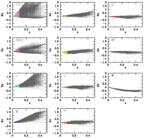
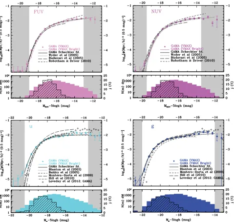
To identify appropriate selection limits we show in Fig. 3 the colour–magnitude diagrams for our data in each band. Following Hill et al. (2010), we identify three obvious selection boundaries for this data set: (1) the limit at which a colour unbiased catalogue can be extracted (long dashed lines); (2) a colour-dependent limit which traces the colour bias (dotted lines); (3) a colour-dependent limit until the mean colour is reached after which a constant limit is enforced (short dashed lines). Volume-corrected luminosity distri-butions can be determined within each of these limits with varying pros and cons. For example while limit 1 offers the simplest and most secure route it uses the minimum amount of data increasing the random errors and susceptibility to cosmic variance. Limit 2 uses all the data but much of these data lie at very faint flux limits which are prone to large photometric error, and the shape of the boundary renders the results particularly susceptible to the Eddington bias. Limit 3 represents a compromise between utilizing excessive poor quality data and reducing the sample excessively. This limit was adopted in Hill et al. (2010) and we follow this practice here. The relevant limits, resulting sample sizes and spectroscopic complete-ness in each band are shown in Table 2. In Fig. 2 data in the redshift range 0.013<z<0.1 are shown as coloured dots.

3 M E T H O D

3.1 Luminosity distribution estimation

In order to derive volume-corrected luminosity distributions in each band we adopt a standard 1/VMaxmethod; this is preferred over a

step-wise maximum-likelihood method as it can better accommo-date the use of multiple selection limits to overcome colour bias. The standard 1/VMaxmethod (Schmidt 1968) can be used to

cal-culate the volume available to each galaxy based on itsr and X

magnitude limits, i.e.XLim is the brightest of 19.4−(r−X) or XFaintLimit(whereXrepresents FUV, NUV,ugizYJHorK), and the

selected redshift range (0.013–0.1). It is worth noting that because of the depth of the survey and the restricted redshift range that this generally constitutes a volume-limited sample at the bright-end of the recovered luminosity distribution in all bands, typically extend-ing∼2 mag belowL∗. Using the 1/VMaxestimator the luminosity

distribution is given by

φ(M)= CX

η

i=N

i=1

1

Vi

,

where the sum is over all galaxies withM−0.25<Mi<M+0.25,η

is the cosmic variance correction for the combined GAMA data over this redshift range (taken here as 0.85; see Driver et al. 2011, fig. 20), andCXis the inverse incompleteness given byCX= _N(withredshifts)N(all) .

Note that the incompleteness is handled in this simplistic way be-cause it is so low,<3.0 per cent in all bands (see Table 2).

Our 1/VMaxestimator has been tested on trial data and the results

are shown on the main panel of Fig. 3. These data were constructed using an input r-band Schechter function of M_r∗−5 log10h = −20.5,α= −1.00 andφ∗=0.003 (Mpch−1)−3, and used to popu-late a 125deg2_{volume toz=0.1. Colours were allocated assuming}

a Gaussian colour distribution with offset (X−r)=3.00 and_σ= 1.00. The test sample was then truncated torKron<19.4 mag and the

method described above used to recover the luminosity distribution

Table 2. Data selection process. Column 2 shows the limit above which the sample is entirely free of any colour bias. Column 3 shows the mean colour above this limit and Column 4 shows the derived faint limit which we adopt in our luminosity function (LF) analysis and is defined as the flux at which the sample becomes incomplete for the mean colour. The remaining columns show the sample size, spectroscopic completeness and the final number of galaxies used in the luminosity function calculation once all selection limits are imposed.

Filter Bright limit Mean colour Faint limit No Comp. No (0.013<z<0.1) (AB mag) (X−r) (AB mag) (per cent)

FUV 20.0 2.46±0.86 21.8 21 740 98.2 7210

NUV 19.5 2.01±0.90 21.5 30 247 97.9 7989

u 19.3 1.73±0.58 21.1 48 602 97.8 10463

g 19.0 0.71±0.27 20.1 60 893 97.7 10990

r 19.4 N/A 19.4 80 464 97.0 11032

i 18.0 −0.42±0.09 19.0 77 586 97.1 10609

z 17.5 −0.66±0.16 18.7 72 821 97.3 9756

Y 17.3 −0.75±0.21 18.6 68 156 97.5 9078

J 17.3 −0.98±0.26 18.4 66 249 97.5 8340

H 17.0 −1.29±0.29 18.1 66 428 97.5 8172

K 16.8 −1.33±0.39 18.1 67 227 97.5 7638

(as indicated by the solid red data points in Fig. 3). The figure indi-cates that the luminosity distribution recovered is accurate (within errors) as long as >10 galaxies are detected within a magnitude bin. It is worth highlighting that although the test data were drawn from a perfect Schechter function distribution, the transformation to a second bandpass under the assumption of a Gaussian colour distribution causes the distribution to become non-Schechter like. As a consequence the bright-end of our test data, when shown in the transformed bandpass, is poorly fitted by a Schechter function (as indicated by the dotted line) with implications for the derived luminosity density as discussed in the next section. The rather ob-vious conclusion is that one should not expect a Schechter function to fit in all bandpasses as the colour distribution between bands essentially acts as a broad smoothing filter. This is compounded by variations in the colour distribution with luminosity/mass and type as well as the impact of dust attenuation which will likewise smear the underlying distributions in the bluer bands (see Driver et al. 2007).

Finally we note that the method described above manages the colour bias by increasing or reducing the 1/VMax

weight-ing accordweight-ing to each objects colour. This will ultimately break-down at the low-luminosity end when a galaxy of a specific colour becomes entirely undetectable at our lower redshift limit of z ∼ 0.013. We can estimate this limit by asking what is the absolute magnitude of a galaxy with the bright limit indicated in Table 2 located atz=0.013. These values are:−13,−13.5,−13.5,−14,−14,−15,−15.5,−15.8,−15.8,−16 and−16.2 forFUV,NUV,ugrizYJHK, respectively, and we adopt these faint absolute magnitude limits when fitting for the Schechter function parameters.

3.2 Luminosity density (jλ)

In this paper we derive two measurements of the luminosity density. The first is from the integration of the fitted Schechter function and the second is from a direct summation of the 1/VMaxweighted fluxes.

Both methods have their merits and weaknesses.

Method 1. Schechter function fitting: The 1/VMaxdata are fitted

by a simple three-parameter Schechter function (Schechter 1976) via standardχ2_{-minimization. The luminosity density is then}

de-rived from the Schechter function parameters in the usual way

[jX = φ∗XLX∗(αX+2) where Xdenotes filter]. This is perhaps

the most standard way of calculating the luminosity density, but it extrapolates flux to infinitely large and small luminosities. In par-ticular, galaxy luminosity functions often show an upturn at both bright and faint luminosities and unless more complex forms are adopted the faint-end in particular is rarely a good fit (see e.g. the unrestricted GAMAugrizluminosity functions with a focus on the faint-end slopes reported in Loveday et al. 2012). Non-Schechter like form is often seen at the very bright-end as well, particularly in the UV and NIR wavebands (see e.g. Robotham & Driver 2011; Jones et al. 2006). The errors for Method 1 are derived by mapping out the full 1σ error ellipse in theM∗-αplane having already op-timised the normalization at each location within this ellipse. The error is then the largest offset inM∗orαwithin this 1σerror ellipse.

Method 2. 1/VMaxSummation: one can directly sum the 1/VMax

weighted luminosities from the individual galaxies within the se-lection boundaries, i.e. (jX=

_i=N

i=0 10

−0.4(Mi−M)

/Vi). This does

not include any extrapolation but rather assumes that the galaxy luminosity distribution is fully sampled over the flux range which contributes most to the luminosity density. The errors are derived from the uncertainty in the flux measurements which we take from Hill et al. (2010) to be±0.03 mag in thegriz,±0.05 in theuYJHK

bands and±0.1 mag in the NUV and FUV (from the mag error distribution given in theGALEXADVANCEDMATCHV02 catalogue).

For our test data the known value is 3.0×109_L

Mpc−3_and

both methods recover accurate measurements of the underlying luminosity density:

Method 1:

3.03+₋₀0._.20₂₄

×109_L

Mpc−3,

Method 2:

2.97+₋00..1518

×109LMpc−3.

GAMA CSED

3249

Figure 2. The colour distributions for our 11-band data with respect torband. The various lines show the three selection boundaries discussed in the text with the thick medium dashed boundary taken as our final 1/VMaxlimit. Data in the redshift range 0.013<z<0.1 are shown in colour and these are the data used

in this paper to derive the CSED.

3.3 Cosmic energy density ()

Our luminosity densities (j_λ) are by convention quoted in units of L_,λhMpc−3. To convert to an energy density which represents the instantaneous energy production rate we need to multiply by the effective mean frequency of the filter in question (as given by the pivot wavelength,λp). We then convert from solar units (L) to

luminosity units (WHz−1). This is achieved using the formula given below, where the observed energy density,Obs_{, is given in units of}

WhMpc−3_:

Obs= c λjλ10

−0.4(M

,λ−34.10) ₍₁₎

the constant term of 34.10 is that required to convert AB magnitudes to luminosity units (i.e. following the Oke & Gunn 1983 definition of the AB magnitude scale in whichmAB= −2.5log10fν+56.1, i.e.

mAB=0 whenfν=3.631×10−23W m−2Hz−1, andFν=4πd2fν

wheredis the standard calibration distance of 10 pc). The observed

energy density,Obs_{, can be converted to an intrinsic energy density,}

Int_{, using the mean photon escape fraction (p}

esc,λ) defined in Driver

et al. (2008, fig. 3), i.e.

Int₌

Obs

/pesc,λ. (2)

The values adopted for the fixed parameters and their associated errors are shown in Table 3. Note that although the solar abso-lute magnitude is required in equation (1) this is only because of the convention of reporting the luminosity density,j_λ, in units of L_,λMpc−3_{as an intermediary step. We adopt this practice to}

al-low for comparisons to previous work but note that the final energy densities are not dependent on the solar luminosity values used. More formally we define the luminosity density to be

jλ=φ∗10−0.4(M ∗

λ−M,λ)(α+2) (3)

Figure 3. Main panel: an illustration of the accuracy of our luminosity density estimator (1/VMax, red squares) as compared to the input test data (solid black

histogram). Also shown is the standard Schechter function fit. Main panel inset: the 1σ, 2σand 3σerror contours for the best-fitting Schechter function to the 1/VMaxdata. Upper panel: the actual number of galaxies used in the derivation of the luminosity distributions. Upper left: the galaxy number counts prior to

any flux or redshifts cuts (black data points) and after the flux and redshift cuts as indicated in Table 2. Lower left: the colour–magnitude diagram showing the full data set prior to cuts (black dots) and after flux and redshift cuts (coloured dots). The coloured lines denote the various selection boundaries as described in Section 2.2.

Table 3. Various constants required for calculation of the luminosity density and energy densities. Filter Aλ/Ar† λ‡Pivot M‡ pesc

(Å) (AB mag) (per cent)

FUV 3.045 1535 16.02 23±6

NUV 3.177 2301 10.18 34±6

u 1.874 3546 6.38 46±6

g 1.379 4670 5.15 58±6

r 1 6156 4.71 59±6

i 0.758 7471 4.56 65±6

z 0.538 8918 4.54 69±5

Y 0.440 10 305 4.52 72±5

J 0.323 12 483 4.57 77±4

H 0.210 16 313 4.71 82±4

K 0.131 22 010 5.19 87±3

†Values taken from Liske et al. (in preparation).

‡Values taken from Hill et al. (2010) forutoKand for FUV and NUV from http://www.ucolick.org/∼cnaw/ sun.html.

for method 1, whereφ∗,M∗andαare the usual Schechter function parameters, and

jλ= n=i

n=1

(10−0.4(Mi,λ−M)

/VMax,i) (4)

for method 2, whereMirepresents the absolute magnitude of theith

object within the specified flux limits andVMax,iis the maximum

volume over which this galaxy could have been seen.

4 D E R I VAT I O N O F T H E L U M I N O S I T Y D I S T R I B U T I O N S A N D D E N S I T I E S

4.1 Corrections to the data

Before the methodology described in the previous section can be implemented a number of corrections to the data must be made to compensate for practical issues of the observing process and known systematic effects.

4.1.1 Galactic extinction and flow corrections

The individual flux measurements in each band are Galactic ex-tinction corrected using the Schlegel maps (Schlegel, Finkbeiner & Davis 1998) with the adoptedAvterms for the 11 bands listed

in Table 3. The individual redshifts are also corrected for the local flow as described in Baldry et al. (2012). These taper the Tonry et al. (2000) multi-attractor model adopted at very low redshift (z<

0.02) to the cosmic microwave background rest frame out toz=

0.03 (see also Loveday et al. 2012). This correction has no signifi-cant impact on the results in this paper but see Baldry et al. (2012) for discussions on the effect this has on the low-mass end of the stellar mass function.

4.1.2 Redshift incompleteness

GAMA CSED

3251

Figure 4.Thek-corrections in each band for the full GAMA I sample as derived usingKCORRECT(v4.2), and indicating generally well-behaved distributions.

Data in the redshift range 0.013<z<0.1 are shown in colour and represent the data used in this paper to derive the CSED.

Table 4.Luminosity function and luminosity density parameters derived for each waveband as indi-cated.

Filter M∗−5logh φ∗ α JMethod1 JMethod2

(AB mag) (10−2h3Mpc−3) (108LhMpc−3) (108LhMpc−3) FUV −17.12+₋00..0503 1.80+

0.12<

−0.07 −1.14+ 0.03

−0.02 3584+ 27

−53 3649+

99 −102

NUV −17.54+₋00..0403 1.77−+00..0808 −1.17+−00..0202 24.6+−00..0403 24.8+−00..0304

u −18.60+₋00..0303 2.03+ 0.05

−0.08 −1.03+ 0.01

−0.01 2.03+ 0.02

−0.03 2.08+ 0.05 −0.06

g −20.09+₋0₀._.03₀₃ 1.47+₋0₀._.04₀₄ −1.10+₋₀0_..01₀₁ 1.96₋+0_0..03₀₃ 1.98+₋0₀._.05₀₆ r −20.86+₋00..0402 1.24+

0.04

−0.03 −1.12+ 0.01

−0.01 2.27+ 0.02

−0.04 2.29+ 0.06 −0.06

i −21.30+₋00..0303 1.00+ 0.04

−0.03 −1.17+ 0.01

−0.01 2.51+ 0.04

−0.04 2.58+ 0.07 −0.07

z −21.52+₋00..0304 1.02+ 0.03

−0.03 −1.14+ 0.01

−0.01 3.00+ 0.05

−0.05 3.07+ 0.08 −0.09

Y −21.63+₋00..0204 0.98+ 0.03

−0.05 −1.12+ 0.01

−0.02 3.06+ 0.06

−0.05 3.13+ 0.08 −0.09

J −21.74+₋00..0403 0.97+ 0.03

−0.03 −1.10+ 0.01

−0.01 3.45+ 0.05

−0.08 3.55+ 0.10 −0.10

H −21.99+₋00..0303 1.03+ 0.02

−0.03 −1.07+ 0.01

−0.01 5.15+ 0.08

−0.08 5.33+ 0.15 −0.15

K −21.63+₋00..0304 1.10+ 0.03

−0.06 −1.03+ 0.03

−0.06 6.00+ 0.09

−0.13 6.21+ 0.17 −0.17

have an impact at the very faint-end where the volumes sampled are exceptionally small. However, as we shall see the luminosity density is entirely dominated byL∗systems and small variations in the derived luminosity density at the very faint-end will have a negligible impact on the CSED.

4.1.3 Absolute normalization and sample/cosmic variance

In Driver et al. (2011) it was reported that the combined GAMA coverage toz<0.1 is 15 per cent underdense with respect to the SDSS main survey. This was estimated by comparing the number of

r-bandL∗galaxies in the GAMA volume to that in the SDSS Main Survey NGP region. We therefore bootstrap to the larger SDSS area

by rescaling all normalization values upwards by 15 per cent to accommodate for this underdensity. We note that by recalibrating the L∗ density to the SDSS main survey we reduce the cosmic variance in the GAMA regions from 14 per cent to the residual variance of the entire SDSS main survey which is estimated, via extrapolation, to be at the 5 per cent level [see Driver & Robotham (2010) for details].

4.1.4 k- and e-corrections

K-corrections are derived for all galaxies using theKCORRECT(v4.2)

software of Blanton & Roweis (2007). We elect to use only the nine-band matched aperture photometry (i.e. SDSS and UKIDSS nine-bands)

Figure 5. Main panels: the luminosity distribution in the FUV, NUV,ugbands (as indicated) derived via 1/VMax(solid data points) applying the corrections

GAMA CSED

3253

using the appropriate SDSS and UKIDSS bandpasses provided with theKCORRECTsoftware. We then determine thek-corrections in all

11 bands andk-correct to redshift zero. Note that no evolutionary corrections (e-corrections) are implemented as the redshift range is low,z<0.1; this assumption could potentially introduce a small wavelength bias as the FUV, NUV,uand gbands will be most strongly affected by any luminosity evolution. Fig. 4 shows thek -correction for our sample. Bimodality is clear in the FUV, NUV and

ubands with values for the FUV becoming quite extreme (∼1 mag) even at relatively low redshift (z∼0.1).

4.2 Global luminosity distributions and densities

The methods of the previous section are now applied to the data resulting in the output shown in Table 4. In all cases the data are well behaved and an acceptable goodness of fit for the Schechter function

parameters is achieved in all 11 bands. Figs 5–7 (main panels) show our recovered luminosity distributions, using our 1/VMaxmethod

and the bright and faint limits reported in Table 2, along with the Schechter function fit to the 1/VMaxfaint-limit data. Previous results

are also plotted, most notably those from theGALEX, Millennium Galaxy Catalogue (MGC), SDSS and UKIDSS surveys. Inugrizwe also include the recent GAMAz<0.1 luminosity functions from Loveday et al. (2012) which use the full GAMA area and original SDSSPetrosianphotometry,k- ande-shifted toz=0. In comparison to this previous GAMA study we generally see good agreement, although on close examination there is a consistent offset at the bright-end with our data shifted brightwards with respect to Loveday et al. (2012). We attribute this to the known difference between Petrosian and Kron photometry for objects with high S´ersic index (see e.g. Graham et al. 2005) which typically dominate the bright-end.

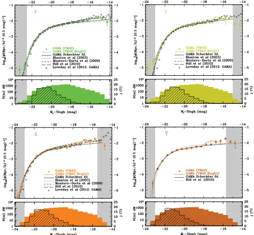
Figure 6. As for Fig. 5 but in therizYbands.

Figure 7. As for Fig. 5 but in theJHKbands.

In comparison to external studies the shape of the curves is mostly consistent with previous measurements with the greatest spread seen in theuandgbands (Fig. 5, lower left and right, respectively). It is important to remember that the GAMA data are, at the bright-end drawn from a volume-limited sample whereas much of the literature values are flux limited. This can have a significant impact on the fitted Schechter function parameters as while the values are unaffected the associated errors will be weighted more uniformly. As a consequence the Schechter function fits are optimized towards intermediate absolute magnitudes over purely flux limited surveys. This subtlety makes it quite tricky to compare Schechter function parameters directly. However, qualitatively the data and fits show very good agreement in all bands and over all surveys.

One feature which is distinctly noticeable is the excess (upturns) at the very faint-end, particularly in the near-IR bands. This has been previously noted in many papers and explored in more detail

for the GAMA data set in theugrizbands by Loveday et al. (2012). The turn-up is most likely brought about by the very red objects at the very bright-end (i.e. elliptical systems) which essentially create a plateau belowL∗ before the more numerous star-forming blue population with an intrinsically steeperα starts to dominate. In all cases the figures show the 1/VMaxresults (which use the limits

given in Table 2, Column 4) as data points and the 1/VMaxbright

results (which use the bright limits given in Table 2, Column 2) as a coloured line. The best-fitting Schechter function (solid black line) is that fitted to the 1/VMaxdata points.

From Figs 5 to 7 the 1/VMax and 1/VMax bright results agree

GAMA CSED

3255

Figure 8.1σconfidence ellipses for the Schechter function fits to the data shown in Figs 5–7.

bright-end indicates where fewer than 10 galaxies are contributing to the recovered luminosity distribution for that bin, and the grey shading at the faint-end indicates where colour bias will commence (see the concluding part of Section 3.1)

In this paper we are primarily interested in the integrated luminos-ity densluminos-ity rather than the luminosluminos-ity functions themselves in order to create the CSED. In all cases we see that the main contribution to the luminosity density (see shaded histograms in lower panels of Figs 5 to 7) stems from aroundL∗, with a minimal contribution from very bright and very faint systems. A key concern might be whether there exists a significant contribution from any low-surface bright-ness systems not identified in the original SDSS imaging data. This seems unlikely as the contribution to the integrated luminosity den-sity falls off at brighter fluxes than where surface brightness issues are expected to become significant (Mr∼ −17 mag). This confirms

the conclusions made in Driver (1999) and Driver et al. (2006) that, while low-surface brightness galaxies may be numerous at very low luminosities, they contribute a negligible amount to the integrated luminosity densities at low redshift.

Fig. 8 shows the associated 1σ error ellipses for the 11-band Schechter function fits. A faint-end slope parameter ofα= −1.11± 0.036 appears to be consistent with all the error ellipses although some interesting trends are seen with wavelength. These trends could be random but could also represent some faint-end incom-pleteness in theuandK bands. This is because as one typically moves away from the selection filter (r) one samples a narrower range in absolute magnitude and less into the faint-end upturn which no doubt influences the values ofα. However, even at its steepest the relatively flat slope ofα= −1.11 implies that relatively little flux density lies outside the fitted range (as indicated by the shaded histograms in Figs 5–7) and that our luminosity density estimates should be robust.

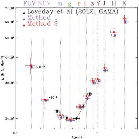
As described in Section 3 the luminosity density is measured in two ways and both of these measurements are shown in Fig. 9 and reported in Table 4. Also shown as joined black data points are the luminosity density values derived by Loveday et al. (2012) which agree extremely well as one would expect. Note that these

1 1

. 0

Figure 9. The luminosity density in solar units as measured through the 11 bands via the two methods. The FUV and NUV data points have been scaled as indicated. The data agree to within the errors in all cases. Method 2 is the preferred method now carried forward. Note the data have been jittered slightly in wavelength for clarity. Also shown are the values taken from Table 6 (i.e. [Column 3+7×Column 4]/8) of Loveday et al. (2012) derived for the0.1_{(ugriz) filter set.}

data are shown offset in wavelength as the values were derived for filtersk-corrected toz=0.1. Reassuringly, the two measurements from the distinct methods agree within their quoted errors in all 11-bands implying that there is no significant error in comparing data derived via alternative methods. This is because the luminosity dis-tributions are well sampled around the ‘knee’ and exhibit relatively modest slopes implying little contribution to the luminosity den-sity in all bands from the low-luminoden-sity population (as discussed above). Although we have made the case that the contribution to the luminosity density is well bounded we acknowledge that the principal caveat to our values is the accuracy and completeness of the input catalogue which can only be definitively established via comparison to deeper data. As the GAMA regions will shortly be surveyed by both VST and VISTA as part of the KIDS and VIKING ESO Public Survey Programs, we defer a detailed discussion of the possible effects of incompleteness and photometric error to a future study.

4.3 The observed GAMA CSED

We now adopt the luminosity density derived from summation of the individual 1/VMaxweights for each galaxy, i.e. Method 2. In Fig. 10

we compare these data to previous studies, most notably Hill et al. (2010) based on the Millennium Galaxy Catalogue showing data from uto K, Blanton et al. (2003) and Montero-Dorta & Prada (2009) which show results from the SDSS fromutoz, Jones et al. (2006) inbJrFJK, and Wyder et al. (2005) and Robotham & Driver

(2011) in the FUV and NUV. Other typically older data sets are also shown as indicated in the figure. Note that these data are now expressed as observed energy densities (i.e.Obs_{; see Section 3.3)}

in which the dependency on the solar SED is divided out, hence

Figure 10. TheobservedCSED from various data sets as indicated. The new GAMA data (black squares joined with dotted lines) are overlaid and the 1σ errors connected via dotted lines which highlight the significant improvement in the uncertainty over the previous compendium of data.

the change in shape from Fig. 9 to Fig. 10. The new GAMA data agree extremely well with previous studies but show considerably reduced scatter (dotted lines) across the UV/optical and optical/NIR boundaries. The crucial improvement is that all the data are drawn from an identical volume with consistent photometry and therefore robust to wavelength-dependent cosmic variance. In comparison to the previous compendium of data the GAMA CSED provides at least a factor of 5 improvement and exhibits a relatively smooth distribution.

Perhaps the most noticeable feature in our CSED is the apparent decline across the transition from the optical to near-IR regime rem-iniscent of the discontinuity seen in the earlier study by Baldry & Glazebrook (2003). Fig. 11 shows the GAMA CSED with thez=

0 model from fig. 12 of Somerville et al. (2012) overlaid (red line), and the same model arbitrarily scaled-up by 15 per cent (blue line). The figure highlights the apparent optical/near-IR discontinuity with the unscaled model (red line) matching the near-IR extremely well while the scaled model (blue line) matches the optical regime very well. It is difficult to understand the source of this uncertainty at this time. The two obvious possibilities are a problem with the data or a problem with the models. The GAMA CSED has been designed to minimize cosmic variance across the wavelength range by sampling an identical volume. Similarly great effort has gone into creating matched aperture photometry fromutoK(Hill et al. 2011) to min-imize the photometric uncertainties. It is also clear that the GAMA

LFs are fully consistent with previous measurements, only a few magnitudes deeper (as indicated by the shaded regions in Figs 5 to 7). In all cases the calculation of the luminosity density is well defined and Fig. 9 demonstrates that the precise method for mea-suring the CSED is not particularly critical with the data generally agreeing within the errors for both methods (which include meth-ods which extrapolate and methmeth-ods which do not). Also the GAMA CSED measurements all lie within the scatter from the compendium of individual measurements shown in Fig. 10. Moreover theYband sits on a linear interpolation between thezandJ bands. Without theY-band data one would infer a sharp discontinuity between the

zandJbands; however because theY band perfectly bridges the disjoint it suggests that the decline is a real physical phenomenon.

GAMA CSED

3257

Figure 11.TheobservedCSED from the GAMA survey with other data shown in grey. Overlaid is the model shown in fig. 12 of Somerville et al. (2012) unscaled and scaled up by 15 per cent.

the required offset between the red and blue curves would likely be much greater. The behaviour of the TP-AGB is also known to be strongly dependent on the metallicity with the progression through the AGB phase significantly faster for lower-metallicity stars. For exceptionally low metallicity systems the third dredge-up can be bypassed entirely, shortening the time over which a TP-AGB star might contribute significantly to the global SED. We defer a detailed discussion of this issue but note the suitability of the GAMA data for either collective or individual SED studies which extend across the optical/near-IR boundary.

5 C O R R E C T I N G F O R D U S T AT T E N UAT I O N

The GAMA data shown in Fig. 10 are all drawn from an identi-cal volume and therefore robust to cosmic variance as a function of wavelength. We therefore ascribe the variation between GAMA data and previous data, in any particular band, as most likely due to cosmic variance (and in particular variations in the normalization estimates of the fitted luminosity functions). The curve and its in-tegral represent the energy injected into the IGM by the combined nearby galaxy population, and is therefore a cosmologically inter-esting number. However, this energy has been attenuated by the internal dust distribution within each galaxy. In a series of earlier papers (Driver et al. 2007, 2008) we quantified the photon escape fraction for the integrated galaxy population when averaged over all viewing angles. This was achieved by deriving the galaxy luminos-ity function in theBband for samples of varying inclination drawn from the Millennium Galaxy Catalogue (Liske et al. 2003). The observed trend ofM∗with cos(i) was compared to that predicted by the sophisticated dust models of Tuffs et al. (2004, see also Popescu et al. 2011) and used to constrain the only free parameter, the face on central opacity, toτBf =3.8±0.7. In Driver et al. (2008) this

value was used to predict the average photon escape fraction as a function of wavelength (0.1–2.1μm) and the values adopted are shown in Table 3. The errors are determined from rederiving the average photon escape fraction using the upper and lower_τBfvalues. These corrections are shown in the final column of Table 3 and are only applicable to the disc populations (i.e. Sabc and later).

Figure 12. The rest-frame (NUV−r) colour for galaxies with secure red-shifts lying in the range 0.013<z<0.1.

In order to accurately correct the CSED for dust attenuation we need to isolate the elliptical population currently believed to be dust free. Rowlands et al. (2012) recently reported that less than 5 per cent of their elliptical sample were directly detected in the far-IR

Herschel-Atlas survey and when far-IR images of the remaining 95 per cent were stacked the flux recovered implied a mean dust mass of less than 106_M

. Hence while not entirely dust free this work suggests they are certainly between 100 and 1000 times dust deficient when compared to similar stellar mass spiral systems. The approach we take to isolate the ellipticals is informative and therefore described in full here. First we attempted to isolate the ellipticals by colour alone. Fig. 12 shows the rest-frame (NUV− r) colour versus redshift in the range 0.013<z<0.1 which show clear bimodality. Selecting a constant division of (NUV−r)z=0=

4.4 mag we repeat the analysis of the previous section to derive the Schechter function parameters and luminosity distribution using our 1/VMaxmethod (see Fig. 13).

The derived luminosity distributions show an interesting effect in that the red population is clearly bimodal with luminosity, exhibiting faint-end upturns in most bands. Inspection of the data suggests that a simple colour cut is overly crude and a significant fraction of edge-on dusty spirals are being included in the red sample and responsible for these upturns. We conclude that colour is not a good proxy for galaxy type. In our second attempt we examine the colour–S´ersic index plane previously highlighted by Driver et al. (2005) as a better discriminator of elliptical systems than colour alone. The S´ersic indices are derived via GAMA-SIGMA (Kelvin et al. 2012, an automated wrapper for GALFIT3, Peng et al. 2010). The fitting process for the GAMA sample is described in detail in Kelvin et al. (2012). Fig. 14 shows the distribution in the colour– S´ersic plane for those galaxies with secure redshifts in the range of interest (0.013<z<0.1) and flux limited torKron<19.4 mag. This

sample contains 10 204 galaxies and exhibits significant structure. Most noticeable are the two dense cores indicated by the two black crosses [n=1, (NUV−r)z=0=2 andn=3.5, (NUV−r)z=0=

5.5] aligned with the anticipated locations of red elliptical and blue discs. The two populations clearly overlap and so we resort to a visual inspection of all systems with (NUV−r)_>3.5 mag orn_>

2. If an object has no recordedNUVflux it is deemed red and added to the elliptical/Spheroid-dominated class.

In Fig. 14 objects classified as elliptical/Spheroid-dominated are indicated by a red cross (1821 systems), those eyeballed but deemed to be not elliptical as green dots (2952), and those not inspected as grey dots (5431). The criteria used in the visual in-spection of the colour postage stamp images are that a galaxy should be concentrated, smooth and ellipsoidal in shape with no indication of internal dust attenuation, no non-uniformity of colour and no tidal stream/plume – all of which might be indicative of a discy (and therefore dusty) system. Eyeball classification is by

definition subjective; however it is clear from the distribution of the two populations that no definitive objective measure will separate the elliptical/Spheroid-dominated (henceforth spheroidal) popula-tion effectively. We do note that a S´ersic index (vertical) cut would appear to be more effective than a colour (horizontal) cut alone. This is primarily because of the colour confusion between old stellar pop-ulations in spheroidal systems and edge-on dust attenuated spirals. More complex automated strategies to morphologically classify the GAMA galaxies will be pursued in future papers once the higher quality imaging data become available.

We now re-derive the luminosity functions (Fig. 15) in each band for the spheroidal (red data and lines) assumed to be devoid of dust, and the remaining populations (blue lines) susceptible to intrinsic dust attenuation. Compared to Fig. 13 the bimodality in the red population is significantly less apparent suggesting that the eyeball

classification is less ambiguous than a simple colour cut. Tables 5 and 6 show the individual Schechter function data for the spheroidal and discy (non-spheroidal) populations, respectively, along with their integrated luminosity densities. We are now in a position to dust correct the spiral population and sum with the as-observed spheroidal population to provide the overall CSED corrected for dust attenuation.

6 T H E E N E R G Y B U D G E T

Table 7 and Fig. 16 show the final CSED values from FUV through to theKband both pre- (upper) and post- (lower) dust attenuated. There are two main motivations for having constructed these data. The first is to provide an estimate of the energy production rate in the Universe today pre-dust attenuation, and the second is to constrain

GAMA CSED

3259

Figure 14. All galaxies withn>2 or (NUV−r)z=0 >3.5 have been

visually inspected. Those deemed ellipticals are indicated by red crosses and those considered not elliptical as green dots. The figure indicates that the S´ersic index is a better indicator of galaxy type than colour but that for any strict automated cut there is serious cross-contamination.

models of galaxy formation. We defer a detailed discussion of the latter to a companion paper which introduces the two-phase galaxy formation model (Driver et al. 2012). However before calculating the pre- and post-corrected energy density we first digress to provide an independent estimate of the local star formation rate from our dust-corrected FUV luminosity density.

6.1 The local star formation rate

The dust-corrected FUV luminosity density is recognized as a good proxy for the star formation rate at the median redshift of the study concerned. This is because typically only massive stars with lifetimes less than 10 Myr contribute significant FUV flux. Fol-lowing Robotham & Driver (2011) we use the standard Kennicutt (1998) prescription based on a Salpeter (1955) initial mass-function, whereby SFRFUV(Myr−1) = 1.4 × 10−28Lν(erg s−1Hz−1)

or 1.4 × 10−28Intλp

10−7_c to derive a star formation rate at a

volume-weighted redshift of z = 0.078 of 0.034 ± 0.003(Ran-dom)±0.009(Systematic, Dust)±0.002(Systematic, cosmic vari-ance) h Myr−1_Mpc−3_{. This is consistent with the compendium}

of results shown in table 4 of Robotham & Driver (2011) and only∼9 per cent higher than the most recent values derived by Wyder et al. (2005) and Robotham & Driver (2011) of 0.0311± 0.006 and 0.0312±0.002hMyr−1_Mpc−3_{, respectively.}

Essen-tially all the star formation is in the non-spheroidal systems and although formally there is 2.7×10−4hMyr−1Mpc−3 in the spheroid population it is highly likely that this flux might be domi-nated by a small number of blue spheroids (see Fig. 14).

6.2 The instantaneous energy output of the nearby Universe

Of cosmological significance is thetotal amount of starlight be-ing produced in the local Universe at the present epoch and the amount which escapes into the IGM and is detectable in UV-NIR

bandpasses. The discrepancy between the energy generated and that which escapes into the IGM in the optical/near-IR window must equate to the local far-IR dust emission if starlight is the only source of heating. The implicit assumption being that the missing light is being attenuated by dust.

To evaluate the energy within the pre-attenuated CSED we must identify a suitable fitting function with which to represent the data. This will enable an extrapolation over the full UV to mid-IR regime. To do this we adopt the predicted spheroid and disc CSEDs from the zero-free parameter two-phase galaxy formation model of Driver et al. (2012) and renormalize them slightly to better fit the data. The renormalized model CSEDs are shown in Fig. 16 (lower panel) as the red and blue curve (for spheroids and discs), and provide a very good match to the data (although note once again the difficulty in matching the sharp decline in the CSED at the optical/near-IR boundary; see discussion in Section 4.3). For full details of these models see Driver et al. (2012); but in brief they adopt a distinct CSFH for spheroids and discs, an evolving metallicity, thePEGASE

star formation code and a Baldry & Glazebrook (2003) IMF. We now integrate the models which include extrapolation to the Lyman limit. We find a total intrinsic energy density of: (1.8± 0.3)×1035_{W h Mpc}−3_{. This is subdivided into an energy budget}

of (1.45±0.2)×1035_{and (0.8±0.1)×10}35_{W h Mpc}−3_{for the}

non-spheroid population before and after attenuation, and (3.6± 0.5) ×1034 _{W h Mpc}−3 _{for the Spheroid population. The final}

errors in the dust-corrected data are almost entirely dominated by the uncertainty in the photon escape fraction (see Table 3, Column 5). Our new local (<z>∼0.078) energy production values (Int_{) can}

be compared to our earlier estimate in Driver et al. (2008) ofInt₌

(1.6±0.2)×1035_{W h Mpc}−3_{. These integrated energy values also}

agree within the errors to the fairly broad ranges deduced in Baldry & Glazebrook (2003) of (1.2–1.7)×1035_{W h Mpc}−3_{for attenuated}

starlight of which (0.3–0.7)×1035_{W h Mpc}−3_{is reprocessed by}

dust.

6.3 Predicting the local far-IR emission

The difference between the total post- and pre-attenuated energies is presumed to be re-radiated in the far-IR by dust grains and equates to a total energy of (6± 1)×1034 _{W h Mpc}−3 _atz

<0.1, i.e. (35±3) per cent of the energy produced by stars is extracted by dust and reradiated in the far-IR [slightly lower than our previous estimate of (43±5) per cent; Driver et al. 2008]. Assuming that the attenuated starlight is entirely absorbed by dust and dominates over all other dust heating processes we can use this value to predict the far-IR CSED. To do this we adopt the average of the Dale & Helou (2002) models 34 and 42, following Baldry & Glazebrook (2003) and Driver et al. (2008). We then renormalize the dust emission curve until it contains the same amount of energy as that lost to the attenuation of stellar light. The attenuated starlight CSED and dust emission CSED can then be added to provide a complete description of the CSED from the Lyman limit (0.1μm) to the sub-mm (<1 mm) wavebands. This wavelength regime is crucial as it entirely dominates the energy production budget of the nearby Universe. The full 0.1μm–1mm CSED is shown in the lower panel of Fig. 16 (black curve) and represents a prediction of the full CSED based on the GAMA UV/optical/near-IR data coupled with the photon escape fractions given in Driver et al. (2008).

In Table 8 we show how our prediction compares to the cur-rently available data from various mid- and far-IR studies. For com-pleteness the actual values and their sources are also shown in Ta-ble 8. These data include the recent estimates in the far-IR from the

Figure 15. Total luminosity functions and those divided by eye into Spirals (blue points and lines) and ellipticals (red points and lines) across the 11 bands as indicated. The eyeball selection on a colour–S´ersic index plane is shown in Fig. 14.

Herschel-Atlas survey (Eales et al. 2010) and derived from the same data set used by Bourne et al. (2012) in generating their table 1. The galaxies from Bourne et al., in the redshift range 0.01<z<0.12, werek- ande-corrected to redshift zero. Thek- ande-corrections were derived from the stacked data and then applied to each indi-vidual galaxy prior to stacking:k-corrections were derived from the shape of the stacked SED in the redshift bin, whilee-corrections were based on the evolutionary fit to luminosities in five redshift bins atz<0.35, given byL(z)∝(1+z)4_{. Following the stacking}

of all optically detected galaxies we obtain fluxes of (5.6±0.4)× 1033_WMpc−3_h

100at 250μm, (2.1±0.1)×1033WMpc−3h100at

350μm and (6.1±0.4)×1032_WMpc−3_h

100at 500μm. Although

these values potentially miss a small amount of faint emission the expectation is that this will be within the errors. The errors quoted include errors from the stacking process and a systematic error of 7

per cent due to the SPIRE flux calibration uncertainty (see Pascale et al. 2011).

The match between our predicted far-IR CSED and the available data is remarkably good, and corroborates our earlier conclusion (Driver et al. 2008) that at low redshift (z<0.1) the dominant source of dust heating is from attenuated starlight which is reradiated in the far-IR.