Robust Tests for a Linear Trend with an Application to Equity
Indices
∗Sam Astilla, David I. Harveyb, Stephen J. Leybourneb and A.M. Robert Taylorc
a. Department of Economics, University of Warwick.
b. Granger Centre for Time Series Econometrics and School of Economics, University of Nottingham.
c. Essex Business School, University of Essex.
February 2014
Abstract
In this paper we develop a testing procedure for the presence of a deterministic linear trend in a univariate time series which is robust to whether the series is I(0) or I(1) and requires no knowledge of the form of weak dependence present in the data. Our approach is motivated by the testing procedures of Vogelsang [1998, Econometrica, vol 66, p123-148] and Bunzel and Vogelsang [2005, Journal of Business and Economic Statistics, vol 23, p381-394], but utilises an auxiliary unit root test to switch between critical values in the exact I(1) and I(0) environments, rather than using this unit root test to scale the test statistic as is done in the aforementioned procedures. We show that our proposed tests have uniformly greater local asymptotic power than the tests of Vogelsang (1998) and Bunzel and Vogelsang (2005) when the error process is exact I(1), identical local asymptotic when the error process is I(0), and have better overall local asymptotic power when the error process is near I(1). Our proposed tests also display superior finite sample power to the tests of Vogelsang (1998) and Bunzel and Vogelsang (2005) and are competitive in finite samples with tests designed to be optimal in both the exact I(1) and I(0) environments. We apply our test procedures to a number of equity indices and find that these series appear to have a significant upward deterministic trend, yet are also highly persistent about this long run growth path.
Keywords: Linear trend, unit root tests, strong serial correlation.
JEL Classification: C22.
∗We thank the Guest Editors, Richard Baillie and Menelaos Karanasos, and two anonymous referees for helpful
1
Introduction
The ability to detect the presence and magnitude of a deterministic trend in an economic time series is of key importance when conducting empirical analysis, the presence of a linear trend being of
particular relevance for the purpose of forecasting or testing for the presence of a unit root. In the latter case, failure to correctly specify a trend when it is indeed present is known to have an adverse effect, resulting in non-similar and inconsistent tests, as demonstrated by Perron (1998). Similarly,
the power of unit root tests to reject the null under the I(0) alternative when a trend is unnecessarily included in a model specification is reduced, see inter alia Marsh (2009) and Ellliot et al. (1996).
The presence of a deterministic trend in an economic or financial time series can also be of interest in its own right, since a linear trend is compatible with a degree of underlying long run growth in the series. For example, this is of particular interest when considering the long run behaviour of stock
prices and indices, where an underlying upward trend implies a long run average return. Moreover, the outcome of statistical tests of the efficient market hypothesis (EMH) are necessarily contingent
on correct specification of the trend component of prices (or, equivalently, the mean component of returns).
Testing for the presence of a linear trend is complicated by the fact that in practice it is typically not known whether the underlying process is I(0) or I(1). For example, uncertainty as to the degree to which financial markets are efficient suggests that one would not want to make an a priori assumption
regarding the presence or absence of a unit root in the series from the outset. We therefore require tests for a linear trend that are robust to whether a series is I(0) or I(1) when determining whether
a trend is present. There have been a number of papers suggesting testing procedures for detecting a deterministic trend function which are robust to the order of integration of the data including,
inter alia, Vogelsang (1998), Bunzel and Vogelsang (2005), Harveyet al. (2007) and Perron and Yabu (2009). Vogelsang (1998) and Bunzel and Vogelsang (2005) employ an auxiliary unit root test statistic to line up the critical values of at-statistic based on the levels of the data in the exact I(1) and I(0)
environments. The approach taken in Harveyet al. (2007) utilises an auxiliary unit root or stationary test statistic to switch between the optimal trend function test in the exact I(1) and I(0) environments, and, as such, the test achieves the Gaussian asymptotic local power envelope in both cases. Perron
and Yabu (2009) use a “super-efficient” estimate of the autoregressive parameter to construct a GLS based test statistic that also achieves the Gaussian asymptotic local power envelope in both the exact
I(1) and I(0) cases.
Compared to the tests of Harveyet al. (2007) and Perron and Yabu (2009), the tests of Vogelsang (1998) and Bunzel and Vogelsang (2005) have the advantage of better size control in finite samples in
the exact I(1) environment when the errors are i.i.d., albeit at the expense of relatively poor power properties, with the tests of Harvey et al. (2007) and Perron and Yabu (2009) fairly similar in terms
of their overall performance. In the local to I(1) environment the results are less clear, with all tests displaying significant undersize, and no one test dominating in terms of overall power.
and Vogelsang (2005) in which an auxiliary unit root test statistic is used to scale the critical value
of the test rather than the test statistic itself. We find the proposed modification yields a test that has uniformly greater local asymptotic power than the tests of Vogelsang (1998) and Bunzel and Vogelsang (2005) when the error process is exact I(1), has identical local asymptotic power when the
error process is I(0) and has better overall finite sample properties. We also find that the proposed tests are competitive in finite samples when compared to the optimal tests of Harvey et al. (2007)
and Perron and Yabu (2009).
The paper is organised as follows. Section 2 outlines the model. Extant tests for a deterministic linear trend are outlined in Section 3. In section 4 we outline our proposed tests. In section 5 the
limiting distribution and local asymptotic power of the tests are detailed. Section 6 reports results of Monte Carlo simulations performed in order to assess the finite sample size and power properties
of the proposed tests relative to existing tests. Section 7 reports results of an empirical exercise in which we apply the test statistics outlined in this paper to a number of US and UK equity indices.
Concluding remarks are made in section 8.
2
The Linear Trend Model
Consider a sample of T observations generated according to the following data generating process (DGP)
yt = µ+βt+ut, t= 1, ..., T (1) ut = αTut−1+εt, t= 2, ..., T. (2)
Following Vogelsang (1998), Bunzel and Vogelsang (2005) and Harvey et al. (2007) we assume that the process{εt} is such that
εt=C(L)et, C(L) := ∞ X
i=0 CiLi
withC(z)6= 0 for all|z| ≤1 andP∞
i=0i|Ci|<∞, and where{et,Ft}is a martingale difference sequence
with E(e2
t|Ft−1) = 1 and suptE(e4t|Ft−1) < ∞. We also define ωε2 := limT→∞T−1E(PTt=1εt)2 = C(1)2. The initial condition,u1, is assumed to beOp(1). These assumptions ensure that we can apply
a Functional Central Limit Theorem (FCLT) to the partial sums of {εt}, so that T−1/2P⌊rTt=1⌋εt →d ωεw(r) where ⌊.⌋ denotes the integer part of its argument, →d denotes weak convergence and w(r) is
a standard Wiener process.
The autoregressive parameter in (2) determines the order of integration of the series. When
αT = α, and |α|< 1 the series is I(0), whereas if αT = 1−α/T¯ the series is near I(1), with ¯α = 0 corresponding to an exact I(1) process. Under these assumptions a FCLT applies to the partial sum of
{ut}defined as St:=Ptj=1uj. When {ut}is I(0), T−1/2S⌊rT⌋→d σw(r), where σ2:=C(1)2/(1−α)2.
When {ut}is near I(1), T−1/2u⌊rT⌋ d
→ωεwα¯(r), where wα¯(r) := Rr
0 exp(−α¯(r−s))dw(s).
the two-sided alternativeH1 :β6=β0, or against either the right-tailed alternativeH1′ :β > β0 or the
left tailed alternativeH1′′ :β < β0. The leading case of interest is where β0 = 0, so that the null and
alternative hypotheses signify the absence or presence of a linear trend, respectively. When analysing the asymptotic performance of the tests outlined in this paper it will prove useful to consider the
local alternative hypotheses of H10:β =β0+κT−3/2 and H11 :β =β0+κT−1/2, where κ is a finite
constant, with the scalingsT−3/2 and T−1/2 providing the appropriate Pitman drifts under I(0) and
I(1) errors, respectively.
3
Extant Tests
In this section we outline the trend tests of Vogelsang (1998), Bunzel and Vogelsang (2005), Harvey
et al. (2007) and Perron and Yabu (2009), all of which are designed to be robust to both the order of integration of the error process and weak dependence in the shocks.
3.1 Scaled Test Statistics
The tPSW1 statistic of Vogelsang (1998) takes the form
tPSW1 := pβˆ−β0 T−1100s2
z
exp(−cξJ)
where ˆβ is the OLS estimator ofβ from (1) andJ denotes theJ unit root test statistic of Park (1990) and Park and Choi (1988) given by the standard OLS Wald statistic normalised by T−1 for testing
the joint hypothesis γ2 =γ3=...=γ9 in the following regression
yt=α+βt+
9 X
i=2
γiti+ut.
The variance estimator is calculated as s2
z := T−1PTt=1S˜t2 where ˜St denotes the residuals from the
following regression
zt= ˜µt+ ˜β t X
j=1
j+ ˜St, t= 1, ..., T
wherezt:=Pts=1ys.
The tPSW1 statistic has a non-degenerate limiting distribution under both I(0) and I(1) errors. The motivation behind this approach is that if the errors are I(0), J →p 0, leaving the asymptotic distribution of the statistic unaffected by the scaling factor exp(−cξJ), whereas if the errors are near
I(1), J converges to a well defined limiting distribution, allowing the practitioner to choose a value of
cξ that lines up the asymptotic critical values of the test in the I(0) and exact I(1) environments for a given significance level,ξ.
TheDan-J statistic of Bunzel and Vogelsang (2005) is a modified version of thetPSW1test statistic
Kiefer and Vogelsang (2005). Specifically, the statistic is given by
Dan-J := q βˆ−β0
ˆ
ω2
u/PTt=1(t−t¯)2
exp(−c′ξJ)
where the long run variance estimator, ˆωu2, is constructed using the Daniell kernel with a data-dependent bandwidth. The bandwidth is given by max(bT,2), where b = bopt( ˆα¯), in which ˆα¯ :=
T(1−αˆ) with ˆα obtained by OLS estimation of (1) and (2), and bopt(.) is a step function given in
Bunzel and Vogelsang (2005). The test statistic is, again, scaled by a function of the J unit root test statistic of Park (1990) and Park and Choi (1988). The constantc′
ξ is, as in Vogelsang (1998), chosen
such that for a given significance levelξ,Dan-J has the same asymptotic critical value under bothI(0) and exact I(1) errors. The value ofc′
ξ depends on b; Bunzel and Vogelsang (2005) provide a response
surface for determining c′ξ for a given significance level, and b. The critical values for the test also depend onb, and again a response surface is provided by the authors for a variety of significance levels. Because ¯α is not consistently estimated by ˆα¯, Bunzel and Vogelsang (2005) only provide a limiting
distribution forDan-J when it is assumed that ¯αis known in the calculation ofb; that is, whenbopt( ˆα¯)
is replaced by bopt(¯α). Although this strictly means that their asymptotic results are based on the
limiting behaviour of an infeasible test, for the purposes of making comparisons tractable, in what follows the limit distribution forDan-J is that using bopt(¯α).
3.2 Asymptotically Optimal Tests
The zλ statistic of Harvey et al. (2007) employs a switching-based strategy that attains the local
limiting Gaussian power envelope for this testing problem irrespective of whether ut is an exact I(1)
process or isI(0). The test statistic is asymptotically distributed as a standard normal under the null in both cases. It is calculated as
zλ := (1−λ∗)z0+λ∗z1 (3)
where
z0:=
ˆ
β−β0 q
ˆ
ω2
u/PTt=1(t−¯t)2
and z1 :=
ˇ
β−β0 p
ˇ
ω2
v/(T −1)
(4)
and where ˆβ denotes the OLS estimator ofβ from (1) and ˆωu2 is a long run variance estimator formed from ˆut:= yt−µˆ−βtˆ , while ˇβ is the OLS estimator of β from (1) estimated in first differences i.e.
from ∆yt=β+vt, t= 2, ..., T, and ˇω2v is a long run variance estimator based on ˇvt:= ∆yt−βˇ. The
weight function λ∗ is defined as
λ∗ := exp −0.00025
DF-GLSτ
KPSS
2!
(5)
where DF-GLSτ is the with-trend local GLS unit root test statistic of Elliott et al. (1996) andKPSS
Whilst the test based onzλattains the local limiting Gaussian power envelope for the case of either
I(0) or exact I(1) errors, Harvey et al. (2007) show that a modified variant of zλ, denoted zλm2, can
provide a more powerful test thanzλ whenut is near-integrated. This replacesz1 withzm1 2:=δξR2z1
where
R2 :=
ˇ
ω2v T−1σˆ2
u 2
and ˆσu2 := (T−2)−1PT
t=1uˆ2t. Here δξ is a constant chosen such that, at a given significance level ξ, zm2
λ has a standard normal critical value under both I(0) and exact I(1) errors.
The tRQFβ test statistic of Perron and Yabu (2009) takes the form of an autocorrelation-corrected
t-ratio on the OLS estimate ofβ obtained from the quasi GLS regression
yt−α˜MSyt−1 = (1−α˜MS)µ+β[t−α˜MS(t−1)] + (ut−α˜MSut−1), t= 2, ..., T y1 = β+u1.
Here, ˜αMS is defined according to the following truncation rule
˜
αMS :=
(
1 if |α˜TWS −1|< T−1/2
˜
αTWS otherwise
where ˜αTWS is an autocorrelation-robust weighted symmetric least squares estimate of α (based on
the OLS residuals ˆut) with one of two truncations applied as described by Roy and Fuller (2001) and
Roy et al. (2004). We will concentrate only on the truncation rule ˜αTWS = ˜αMU, where ˜αMU is as
described in Perron and Yabu (2009), who show this truncation gives the better finite sample power properties. The tRQFβ statistic is asymptotically standard normal under the null hypothesis when ut
is either I(0) or exact I(1) and, as noted in Remark 2 of Perron and Yabu (2009), has the same local asymptotic power as the zλ statistic of Harveyet al. (2007) in the local-to-unity autoregressive root
environment that we consider in this paper.
4
Modified Tests
Our proposed testing procedure involves utilising similart-ratios to Vogelsang (1998) and Bunzel and Vogelsang (2005), although we propose use of the auxiliary J unit root test to switch between the exact I(1) and I(0) critical values. Such an approach has the advantage that it leads to a test with
local asymptotic power identical to the tests of Vogelsang (1998) and Bunzel and Vogelsang (2005) when the errors are I(0), but with greater local asymptotic power when the shocks are I(1) due to
the removal of the influence of the auxiliary unit root test statistic on the asymptotic distribution of the test in the I(1) case. Specifically, the first test statistic is a modified version of thetPSW1 test of Vogelsang (1998) calculated as
tP SWs1:= pβˆ−β0 T−1100s2
Notice that this is identical to the original tPSW1 statistic of Vogelsang (1998) but excluding the
scaling factorexp(−cξJ). We then calculate the weight function
λ′:=exp(−τ T1/2Jυ) (6)
with constantsυ >0.5 andτ >0, and compare thetP SW1
s test statistic to a critical value,cv, given
by
cv:= (1−λ′)cvI(1)+λ′cvI(0)
where cvI(1) and cvI(0) are the asymptotic critical values of the tP SWs1 statistic at the desired sig-nificance level in the exact I(1) and I(0) environments, respectively. The rationale behind such an
approach is that when the error process,ut, is I(1),Jυ isOp(1), so thatT1/2JυisOp(T1/2) and hence λ′ →p 0 and so the exact I(1) critical value is used. Conversely, whenu
t is I(0),Jυ isOp(T−υ), so that T1/2Jυ is op(1) given υ >0.5, and now λ′ →p 1 so that the I(0) critical value is used. Consequently, at least asymptotically, the test will have correct size regardless of whether the error process is I(0) or exact I(1). This holds irrespective of the values ofτ >0 andυ >0.5, which are calibrated later in
the paper to best control the size of the test in finite samples.1
We also apply the same principle to the test statistic of Bunzel and Vogelsang (2005), with our
proposed test statistic given by
Dan-Js:=
ˆ
β−β0 q
ˆ
ω2
u/PTt=1(t−t¯)2 .
We then calculate the scaling factorλ′ in the same way as previously described and use this to switch
between the relevant critical values in the exact I(1) and I(0) environments. With this procedure the critical values will, as with the test of Bunzel and Vogelsang (2005), depend on the choice of bandwidth,b, used to estimate the long run variance.
5
Asymptotic Results
We now examine the asymptotic behaviour of the test statistics outlined in this paper. We consider the size and power properties of the test under both the null hypothesis H0 : β = β0 and the local
alternative hypothesesH10:β=β0+κT−3/2 andH11:β =β0+κT−1/2, where κis a finite constant,
with the T-scalings providing the appropriate Pitman drift under I(0) and I(1) errors, respectively. The limiting distributions are expressed in terms of the following functions defined below.
1Notice that the required properties for the large sample behaviour ofλ′ under I(0) and I(1) errors are also satisfied
by 1−λ∗, whereλ∗is the weight function (5) used by Harveyet al. (2007). Other specifications forλ′ could also be
used, provided thatλ′ p
→0 under I(1) and λ′ p
→1 under I(0). The weight function adopted in (6) has the advantage
of requiring the computation of only one auxiliary statistic. Moreover, while less parameterized specifications could be adopted, we found that the greater flexibility permitted by the inclusion of υ andτ delivered improved overall finite
Definition 1
F(r) := [1, r]′, G(r) := [r,(1/2)r2]′, Q(r) := [1, r, r2, ..., r9]′, R∗:= [0,1]
NF :=
( R1
0 F(s)dw(s) if |α|<1 R1
0 F(s)wα¯(s)ds if α= 1−α/T¯
H(r) :=
(
w(r) if |α|<1
Rr
0 wα¯(s)ds if α= 1−α/T¯
QF(r) :=H(r)−
Z r 0
F(s)′ds Z 1
0
F(s)F(s)′ds −1
NF
ΦF(b, k) :=
Z 1
0 Z 1
0 −
k′′((r−s)/b)QF(r)QF(s)drds
Ac :=
R1
0 Lc(wα¯(r), F(r))2dr R1
0 Lc(wα¯(r), Q(r))2dr
−1,
wherek′′(x) is the second derivative of the Bartlett kernel andLc(p, q) generically denotes the
contin-uous time residuals from the projection ofp onto the space spanned byq.
Consider first the I(0) case. To that end if yt is generated according to (1) and (2) with |α|<1 and β=β0+κT−3/2, then,
tPSW1, tPSW1s →d
κ/σ+R∗′R1
0 F(s)F(s)′ds −1
NF r
100R1
0 Lc(w(r), G(r))2drR∗
R1
0 F(s)F(s)′ds −1
R∗′
zλ, zmλ2, t RQF β
d
→ w(1) +κ/(√12σ)
Dan-J, Dan-Js →d
κ/σ+R∗′R1
0 F(s)F(s)′ds −1
NF r
ΦF(b, k)R∗R1
0 F(s)F(s)′ds −1
R∗′
The proofs for the tPSW1s and Dan-Js statistics follow trivially from those of the tPSW1 and
Dan-J statistics given in Vogelsang (1998) and Bunzel and Vogelsang (2005). The proofs for the zλ, zm2
λ and t RQF
β tests are taken from Harvey et al. (2007) and Perron and Yabu (2009). The modified
and unmodified versions of the statistics of Vogelsang (1998) and Bunzel and Vogelsang (2005) share the same asymptotic distribution in the I(0) case and, as such, will have the same asymptotic local
Next consider the I(1) case. If yt is generated according to (1) and (2) with α = 1−α/T¯ and β =β0+κT−1/2, then
tPSW1 →d
κ/ωε+R∗′
R1
0 F(s)F(s)′ds −1
NF r
100R1 0 Lc
R1
0 wα¯(s)ds, G(r) 2
drR∗R1
0 F(s)F(s)′ds −1
R∗′
exp(−cξAc)
Dan-J →d
κ/σ+R∗′R1
0 F(s)F(s)′ds −1
NF r
ΦF(b, k)R∗R1
0 F(s)F(s)′ds −1
R∗′
exp(−cξAc)
zλ, tRQFβ d
→ wα¯(1) +κ/ωε zλm2 →d δγ
Z 1
0
Lc(wα¯(r), F(r))dr −2
(wα¯(1) +κ/ωε)
tPSW1s →d
κ/ωε+R∗′R1
0 F(s)F(s)′ds −1
NF r
100R1 0 Lc
R1
0 wα¯(s)ds, G(r) 2
drR∗R1
0 F(s)F(s)′ds −1
R∗′
Dan-Js →d
κ/σ+R∗′R1
0 F(s)F(s)′ds −1
NF r
ΦF(b, k)R∗R1
0 F(s)F(s)′ds −1
R∗′
The proofs for the tPSW1s and Dan-Js statistics, again, follow trivially from those of thetPSW1
and Dan-J statistics given in Vogelsang (1998) and Bunzel and Vogelsang (2005). The proofs for the
zλ,zλm2 andtRQFβ tests are, once again, taken from Harveyet al. (2007) and Perron and Yabu (2009).
As can be seen, the limiting distributions of the modified versions of thetPSW1sandDan-Jsstatistics
now differ from those of the original versions of these statistics. This is due to the fact that the J
unit root test impacts the asymptotic distribution of the original statistics, which will in turn affect their local asymptotic power, whereas for the modified tests this same test statistic is simply used
to select the critical value, which will have no effect on local asymptotic power. The main difference between the modified and unmodified statistics is that the additional variation from theJ unit root test statistic impacts the asymptotic distribution of thetPSW1 andDan-J statistics, whereas for the
tPSW1s andDan-Js statistics this variation impacts the critical value selected asymptotically. In the
exact I(1) case we will show that this leads to large power gains for the modified tests relative to their
unmodified counterparts.
We now examine the asymptotic power functions of all of the above tests by directly simulating the limiting representations given above. The Weiner processes were approximated usingN IID(0,1)
random variates and approximating integrals by normalised sums of 1000 steps. All Monte Carlo simulations that follow were performed in Gauss 9.0 using 10,000 replications. The results we report
are for one-sided tests of H0 : β = β0 against H1′ : β > β0. Consequently, results are reported for
of κ. All results are presented at an asymptotic level of 5%. For the Dan-Js test a bandwidth of b= 0.02 was utilised in all scenarios as this choice of bandwidth led to a test with the greatest local asymptotic power for both I(1) and I(0) errors, as such, we recommend the use of this bandwidth when performing the Dan-Js test in practice and perform the test utilising this bandwidth for the
remainder of the paper. For the Dan-J test results are reported for b =bopt(¯α). Note that all tests
are constructed to give an asymptotic size of 5% in the I(0) and exact I(1) environment, thus for the
case of errors that are near I(1) with ¯α >0 the tests will be conservative.
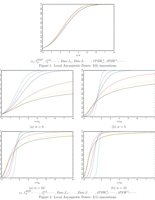
For the case of I(0) errors results are reported for the null hypothesis H0 :β =β0 and the local
alternative H10 : β = β0 +κT−3/2. We consider a range of κ ∈ [0,20] using a grid with 100 steps,
with results reported in Figure 1. As can be seen, the greatest power is achieved by the zλ, zλm2 and tRQFβ tests, with all of these tests attaining the Gaussian asymptotic local power envelope. TheDan-J
andDan-Jstests have identical asymptotic local power functions, as do thetPSW1 andtPSW1s tests.
Although the tests based onDan-J have uniformly better power than the tests based ontPSW1, they
are slightly less powerful than thezλ,zmλ2andtRQFβ tests which are asymptotically optimal in the I(0) environment.
For the case of near I(1) errors results are reported for the null hypothesis H0 :β = β0 and the
local alternative H11 :β =β0+κT−1/2 for a range of ¯α ∈[0,5,10,15], with ¯α = 0 corresponding to
an exact I(1) process. We consider a range ofκ∈[0,8] using a grid with 100 steps. Figure 2(a) shows a clear ordering in the asymptotic local power of the test statistics in the exact I(1) case, with the zλ
and tRQFβ tests achieving the Gaussian asymptotic local power envelope and displaying the greatest overall power. TheDan-Js andtPSW1s tests display power significantly in excess of their unmodified
counterparts, with the zλm2 test attaining power somewhere between the modified and unmodified tests. The superiority of the new modified tests, compared with their unmodified counterparts, is
unsurprising as the choice to utilise the auxiliary unit root test statistic to select the critical value rather than scale the test statistic itself removes the influence of the auxiliary unit root test statistic on the asymptotic distribution of the test in the I(1) case, leading to greater local asymptotic power.
The results are more mixed when ¯α >0, with no single test having uniformly greater power for all values ofκ. Results for ¯α= 5, reported in Figure 2(b), show that all of the procedures are under-sized,
particularly so in the case of the zλ andtRQFβ tests. In this scenario it is, in fact, the originaltPSW1
and Dan-J tests that have the best power properties for values ofκ less than around 1.6, followed by the zm2
λ , tPSW1s and Dan-Js tests, with the zλ and tRQFβ tests having the lowest overall power. For
values ofκ greater than around 1.6, however, the power ordering is reversed, with the tests reverting to the power ordering observed for the exact I(1) case. In particular thezλ,tRQFβ ,Dan-JsandtPSW1s
tests display power significantly in excess of thezmλ2,tPSW1 and Dan-J tests for moderate values of
κ.
The pattern of results for ¯α = 10 and ¯α = 15, presented in Figures 2(c) and 2(d), respectively,
are broadly similar to the case of ¯α = 5, although as ¯α increases the zmλ2 test begins to dominate other tests for values of κ less than around 1.6. Whilst the power ordering is otherwise identical,
around 1.6 is increasing in ¯α, with the power functions of thezλ and tRQFβ tests converging towards
a step function atκ= 1.645 as ¯α is increased.
In summary, if we are interested in only I(0) or exact I(1) processes then thezλandtRQFβ tests have
uniformly greater local asymptotic power. The results are, however, mixed if we allow for the case of
near I(1) processes. The most important point to note, however, is that in the exact I(1) scenario using theJ unit root test statistic to select a critical value in the testing procedure of Vogelsang (1998) and
Bunzel and Vogelsang (2005) rather than scaling the test statistic itself yields substantial power gains, with the tPSW1s and Dan-Js tests displaying power far in excess of the original tPSW1 and Dan-J
tests. For near I(1) processes results are less clear, with the modified versions of the test of Vogelsang
(1998) and Bunzel and Vogelsang (2005) displaying power below their unmodified counterparts for small values ofκ, but displaying greater power for larger values ofκ. It will, therefore, be important
to examine how this pattern of local asymptotic power translates into the finite sample performance of the proposed tests.
6
Finite Sample Simulations
In this section we present the results from a Monte Carlo simulation exercise performed to assess
the finite sample size and power properties of the tests discussed in this paper. Data were generated according to
yt = µ+βt+ut, t= 1, ..., T, ut = αTut−1+et+θet−1,
withet∼N IID(0,1), αT = 1−α/T¯ and u1 =e1 =e0 = 0. We test the null hypothesis H0 :β =β0
against the one-sided alternative H1′ : β > β0, using one-sided tests, and where without loss of
generality we set β0 = µ = 0. All tests were performed at the nominal 5% level. When performing
thetPSW1s and Dan-Js tests values ofτ and υ used when calculating the relevant critical value were
calibrated to give the best overall small sample performance. We considered values of υ = 1 and
υ = 2 and for each test and value of υ a value of τ was chosen such that size was controlled across all scenarios considered. For a givenυ smaller values ofτ lead to a test with higher finite sample size due to more weight being placed on the I(0) critical value, whereas larger values of τ lead to lower
finite sample size as more weight is placed on the I(1) critical value. We found that υ = 2 for both tests and values ofτ = 0.03 andτ = 0.074 for thetPSW1s and Dan-Js tests, respectively, led to tests
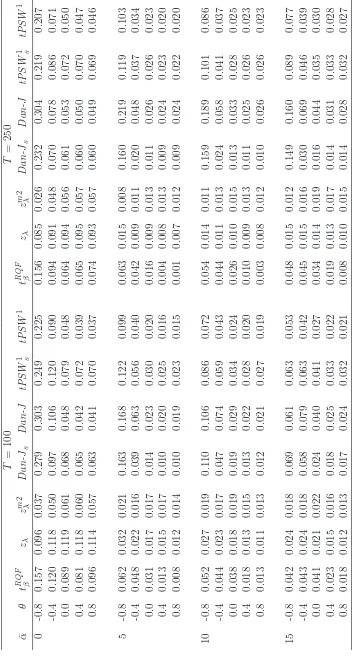
with well controlled size for i.i.d errors in all scenarios and decent finite sample power properties. Table 1 reports the size of the testing procedures for a range of ¯α ∈ [0,5,10,15] and θ ∈
[−0.8,−0.4,0.0,0.4,0.8]. We see that all the tests except the tPSW1 and Dan-J tests have poor size control when ¯α= 0,T = 100 and the errors are i.i.d., with thezλ test displaying the worst overall
size distortions with an empirical size of 11.9%. The tPSW1s and Dan-Js tests are also oversized,
T = 250 but are still noticeable for all but the tPSW1 and Dan-J tests. For the near integrated
scenarios considered, all of the tests are conservative when the errors are i.i.d., with actual size below the 5% nominal level for all values of ¯α >0. Moving away from the i.i.d. case, we see that introducing negative MA behaviour into the noise function leads to an increase in the size of all tests for all values
of ¯α, with the exception of thezλandzλm2 tests. For these two tests size is relatively unaffected by the
value ofθ, with only the caseθ <0 and ¯α= 0 leading to a reduction in size. For the remaining tests,
size distortions are most noticeable for the tests based onDan-J, although the tests based ontPSW1
do suffer quite severe size distortions when ¯α= 0 and θ <0. The size of all tests are less sensitive to positive MA behaviour, with the size of the tests in this scenario almost identical to the i.i.d. case.
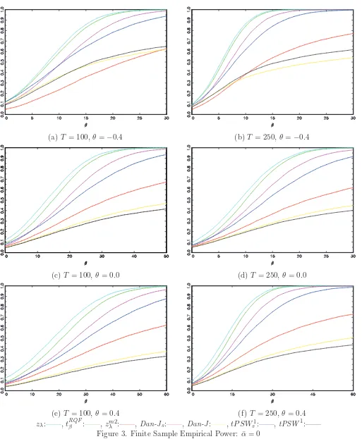
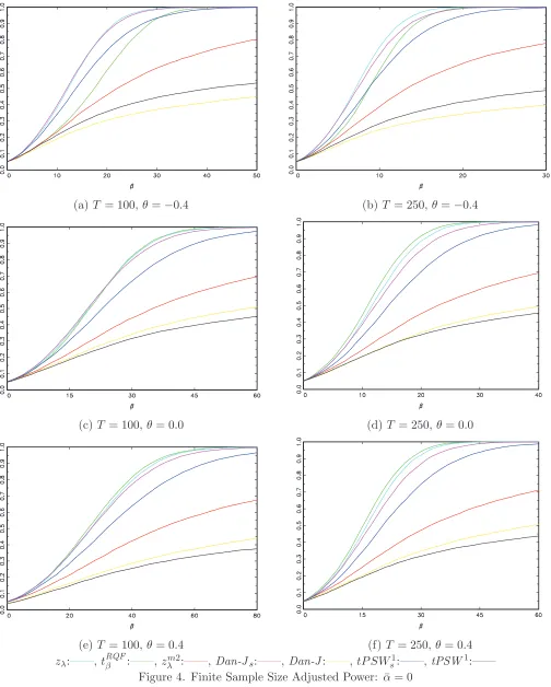
We now turn our attention to the power of the tests under the alternative. Figure 3 reports results for ¯α = 0 for sample sizes ofT = 100 and T = 250 and values of θ∈[−0.4,0.0,0.4]. In this scenario there is a clear ordering in the power of the tests, with zλ having uniformly greater power than all
tests, closely followed by tRQFβ . The tPSW1s and Dan-Js tests have power significantly in excess of
their unmodified counterparts, with power of thezλm2 test somewhere between that of thetPSW1s and the Dan-J test. These results are unsurprising given that the most powerful tests in this scenario are also those that are most oversized. As such, Figure 4 reports size adjusted power for the same
scenarios. For a sample size ofT = 100 with i.i.d. errors the best size adjusted power is given by the
tRQFβ ,zλ andDan-Jstests, with the tPSW1s test the most powerful of the remaining tests. When the
sample size is increased to T = 250 the results are fairly similar, although the tRQFβ test now shows the best power overall, followed byzλ, thenDan-Js. We see a similar pattern of results when we allow
for positive MA behaviour in the error process, although when we allow for negative behaviour when
θ=−0.4 the results are slightly different. In this scenario the best overall power is now achieved by thezλ and Dan-Js tests, followed by the tPSW1s and tRQFβ tests.
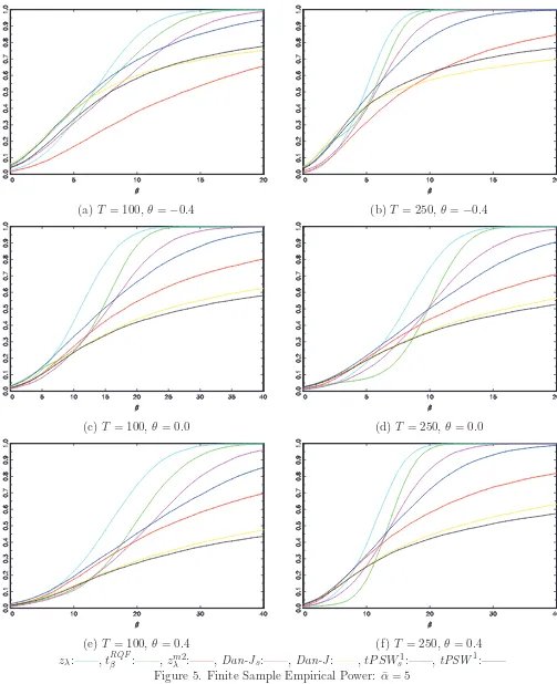
Figure 5 reports the power of the tests for ¯α = 5. In this scenario results are mixed, with the
zλ test displaying arguably the best overall power, although it is somewhat less powerful than the
other tests for smaller values of β, reflecting the local asymptotic power results in Figure 2(b). The
most important results to note in this scenario are that, much like in the case of exact I(1) errors, the
tPSW1s and Dan-Js tests have better overall power than their unmodified counterparts. The power
of the tPSW1s test is uniformly higher than that of the tPSW1 test, and the Dan-Js test is more
powerful than the Dan-J test for all but very small values of β. The tPSW1s test also shows higher power than both the zλ and tRQFβ tests for lower values ofβ.
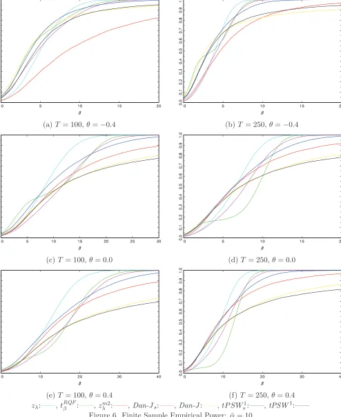
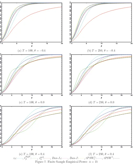
Figures 6 and 7 report the power of the tests for ¯α = 10 and ¯α = 15, respectively. Results here are, once again, rather mixed. The power functions of the tests are much closer together, particularly
for ¯α = 15, with no one test dominating the others. What is important to note, however, is that the
tPSW1s test, once again, shows uniformly greater power than its unmodified counterpart. TheDan-Js
test, however, does not perform so well with the power of this test falling below that of the original
Dan-J test for all but large values of β. The tPSW1s test is again competitive with thezλ and tRQFβ
tests.
at hand. The important result is that the tPSW1s test shows uniformly greater finite sample power than the original tPSW1 test, and often has the best power properties of all tests for smaller values of β and when ¯α > 0. Results for the Dan-Js test are less clear cut. While the power of this test
is greater than both the tPSW1s and Dan-J tests in the exact I(1) environment, it appears to show inferior power properties to these two tests in the near integrated environment.
7
Application to Equity Indices
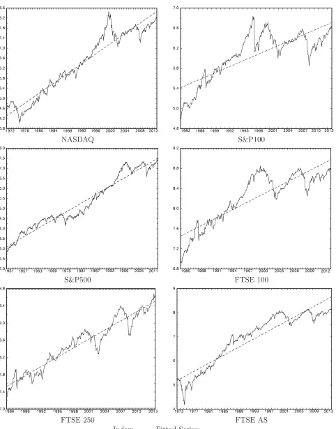
We now apply the test statistics outlined in this paper to a number of stock market indices. We consider the natural logarithm of the monthly closing price of six equity indices using all available
data sourced from Yahoo! finance. The six indices utilised are the NASDAQ (02/1971-10/2013), S&P100 (08/1982-10/2013), S&P500 (01/1950-10/2013), FTSE 100 (04/1984-10/2013), FTSE 250
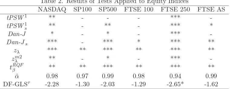
(12/1985-10/2013) and the FTSE All Share (12/1972-10/2013). For each index, Table 2 reports whether one-sided implementations of the tests outlined in this paper reject in favour of a positive trend at the 10%, 5% or 1% significance levels. We also report the associated estimate ofαT obtained
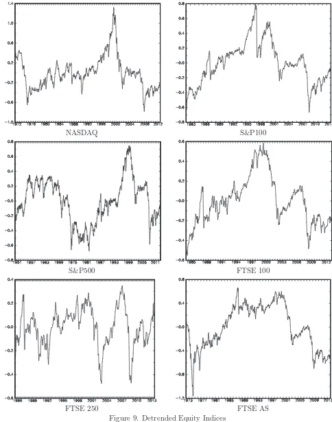
from OLS estimation of (1)-(2), denoted ˆα. Figure 8 plots the series and the fitted deterministic components, whilst Figure 9 plots the detrended series.
The rejection patterns associated with the different tests appear to mirror the asymptotic and finite sample power results reported in Sections 5 and 6. The zλ and tRQFβ tests detect a linear trend
for each of the six equity indices, with thetPSW1s andDan-Jstests indicating trends in four and five,
respectively, of the six series. We note that while thetPSW1s and Dan-Js tests fail to detect a trend
in some cases they do, however, provide more evidence for the presence of a deterministic trend than
their unmodified counterpartstPSW1 and Dan-J; moreover, they never fail to detect a trend where it is detected by the unmodified tests.
For each series, at least one of the tests indicates the presence of a deterministic linear trend, lending strong support to the notion that equity price indices are subject to (positive) long run growth. This implies non-zero long run average returns, and therefore an investment strategy of buy and hold for
an index would be expected to deliver positive returns equal to the long run growth rate. An obvious implication of these findings is that any subsequent tests of the EMH should take account of a long
run trend component in prices (or a non-zero mean component in returns).
Examining the values of ˆα in Table 2 it is seen that the residuals from the detrended series are, in all instances, compatible with processes which are either I(1) or I(0) but highly persistent. As a
further indication as to the integration properties of the data, the with-trend local GLS unit root test statistic of Elliott et al. (1996), DF-GLSτ, is also reported for each series in Table 2. We see from
these results that the unit root null is not rejected at conventional significance levels for five of the six series; for the FTSE 250 index, a rejection is found at the 10% significance level. That there is some modest evidence of stationary, as well as unit root, behaviour across the different series reinforces
asymptotically, we may conclude that deterministic trends are present in these stock indices with a
reasonable degree of confidence, without needing to explicitly model the stochastic component of the series.
8
Conclusions
In this paper we have proposed a modification to the trend tests of Vogelsang (1998) and Bunzel
and Vogelsang (2005) in which a unit root test statistic is used to select the critical value utilised in the trend test procedure rather than being used to scale the test statistic itself, the latter being the approach in Vogelsang (1998) and Bunzel and Vogelsang (2005). We have shown that these modified
tests have uniformly greater local asymptotic power than their unmodified counterparts in the exact I(1) environment and identical local asymptotic power in the I(0) environment, and that the modified
version of the test of Vogelsang (1998) not only has uniformly greater finite sample power than its unmodified counterpart, but also has power in the near I(1) environment that is competitive with the asymptotically optimal tests of Harvey et al. (2007) and Perron and Yabu (2009). That this
modified test is able to dominate the test of Vogelsang (1998) across most scenarios whilst attaining power which is competitive with tests designed to be optimal in the exact I(1) and I(0) environment
is encouraging, and motivates the use of this modification in other testing problems where the test statistic has a different limiting distribution in the I(1) and I(0) environments. In the current context
of testing for a linear trend, applying the tests examined in this paper to a number of equity indices uncovers strong support for the presence of deterministic trends in the series, implying that long run growth represents an important characteristic of such stock price indices.
References
Bunzel, H. and Vogelsang, T.J. (2005). Powerful trend function tests that are robust to strong serial correlation, with an application to the Prebisch-Singer hypothesis. Journal of Business and Economic Statistics 23, 381-94.
Elliott, G., Rothenberg, T.J. and Stock, J.H. (1996). Efficient tests for an autoregressive unit root.
Econometrica 64, 813-36.
Harvey, D.I., Leybourne, S.J., and Taylor, A.M.R. (2007). A simple, robust and powerful test of the
trend hypothesis. Journal of Econometrics 141, 1302-30.
Jansson, M. (2002). Consistent covariance matrix estimation for linear processes. Econometric Theory 18, 1449-1459.
Kwiatkowski, D., Phillips, P.C.B., Schmidt, P. and Shin, Y. (1992). Testing the null hypothesis of stationarity against the alternative of a unit root: how sure are we that economic time series
Kiefer, N. M. and Vogelsang, T. J. (2005). A new asymptotic theory for heteroskedasticity-autocorrelation
robust tests. Econometric Theory 21, 1130-1164.
Marsh, P.W.N. (2009). The properties of Kullback-Leibler divergence for the unit root hypothesis.
Econometric Theory 25, 1662-81.
Park, J.Y. (1990). Testing for unit roots and cointegration by variable addition, in Fomby, T. and Rhodes, F. (eds.) Advances in Econometrics: Cointegration, Spurious Regression and Unit
Roots. Jai Press: Greenwich.
Park, J.Y. and Choi, B. (1988). A new approach to testing for a unit root. CAE Working Paper
88-23, Cornell University.
Perron, P. (1998). Trends and random walks in macroeconomic time series: further evidence from a new approach. Journal of Economic Dynamics and Control 12, 297-332.
Perron, P. and Yabu, T. (2009). Estimating deterministic trends with an integrated or stationary noise component. Journal of Econometrics 151, 56-69.
Roy, A., Falk, B. and Fuller, W.A. (2004). Testing for trend in the presence of autoregressive errors.
Journal of the American Statistical Association 99, 1082-1091.
Roy, A. and Fuller, W.A. (2001). Estimation for autoregressive processes with a root near one.
Journal of Business and Economic Statistics 19, 482-493.
Table 2. Results of Tests Applied to Equity Indices
NASDAQ SP100 SP500 FTSE 100 FTSE 250 FTSE AS
tPSW1 ** - - - ***
-tPSW1s ** - ** - *** *
Dan-J * - * - ***
-Dan-Js *** - *** * *** **
zλ *** ** *** ** *** **
zmλ2 ** - * - ***
-tRQFβ ** ** *** ** *** **
ˆ
α 0.98 0.97 0.99 0.98 0.94 0.99 DF-GLSτ -2.28 -1.30 -2.03 -1.29 -2.65* -1.62
zλ,tRQF
[image:18.595.71.570.98.739.2]β ,zλm2:——,Dan-Js,Dan-J:——,tP SWs1,tPSW1:——
Figure 1. Local Asymptotic Power: I(0) innovations
(a) ¯α= 0 (b) ¯α= 5
(a) ¯α= 10 (b) ¯α= 15
zλ ,tRQF
β :——,z m2
λ :——,Dan-Js:——,Dan-J:——,tP SWs1:——,tPSW1:——
(a) T = 100, θ=−0.4 (b) T = 250, θ=−0.4
(c) T = 100, θ= 0.0 (d)T = 250, θ= 0.0
(e) T = 100, θ= 0.4 (f) T = 250, θ= 0.4
zλ:——,tRQF
β :——,z m2
[image:19.595.68.581.106.729.2]λ :——,Dan-Js:——,Dan-J:——,tP SWs1:——,tPSW1:——
(a) T = 100, θ=
−0.4 (b) T = 250, θ=−0.4
(c) T = 100, θ= 0.0 (d)T = 250, θ= 0.0
(e) T = 100, θ= 0.4 (f) T = 250, θ= 0.4
zλ:——,tRQF
[image:20.595.69.573.108.736.2]β :——,zλm2:——,Dan-Js:——,Dan-J:——,tP SWs1:——,tPSW1:——
(a) T = 100, θ=−0.4 (b) T = 250, θ=−0.4
(c) T = 100, θ= 0.0 (d)T = 250, θ= 0.0
(e) T = 100, θ= 0.4 (f) T = 250, θ= 0.4
zλ:——,tRQF
β :——,z m2
[image:21.595.66.569.111.729.2]λ :——,Dan-Js:——,Dan-J:——,tP SWs1:——,tPSW1:——
(a) T = 100, θ=−0.4 (b) T = 250, θ=−0.4
(c) T = 100, θ= 0.0 (d)T = 250, θ= 0.0
(e) T = 100, θ= 0.4 (f) T = 250, θ= 0.4
zλ:——,tRQF
β :——,z m2
[image:22.595.74.568.120.724.2]λ :——,Dan-Js:——,Dan-J:——,tP SWs1:——,tPSW1:——
(a) T = 100, θ=−0.4 (b) T = 250, θ=−0.4
(c) T = 100, θ= 0.0 (d)T = 250, θ= 0.0
(e) T = 100, θ= 0.4 (f) T = 250, θ= 0.4
zλ:——,tRQF
β :——,z m2
[image:23.595.69.574.109.730.2]λ :——,Dan-Js:——,Dan-J:——,tP SWs1:——,tPSW1:——
NASDAQ S&P100
S&P500 FTSE 100
FTSE 250 FTSE AS
[image:24.595.70.552.99.714.2]NASDAQ S&P100
S&P500 FTSE 100
[image:25.595.62.546.112.727.2]FTSE 250 FTSE AS