Duality based two level error estimation for time dependent PDEs: application to linear and nonlinear parabolic equations

Duality-Based Two-Level Error Estimation for

Time-Dependent PDEs:

Application to Linear and Nonlinear

Parabolic Equations

G. S¸im¸sek

, X. Wu

, K.G. van der Zee

, E.H. van Brummelen

_,

5600 MB Eindhoven, Netherlands

††_{School of Mathematical Sciences, The University of Nottingham University Park,}

Nottingham NG7 2RD, United Kingdom

Abstract

We introduce a duality-based two-level error estimator for linear and nonlinear time-dependent problems. The error measure can be a space-time norm, energy norm, final-time error or other error related functional. The general methodology is developed for an abstract nonlinear parabolic PDE and subsequently applied to linear heat and nonlinear Cahn–Hilliard equations. The error due to finite element approx-imations is estimated with a residual weighted approximate-dual solution which is computed with two primal approximations at nested levels. We prove that the exact error is estimated by our estimator up to higher-order remainder terms. Numerical experiments confirm the theory regarding consistency of the dual-based two-level es-timator. We also present a novel space-time adaptive strategy to control errors based on the new estimator.

Contents

1 Introduction 2

2 Duality-Based Two-Level Error Estimation 4

2.1 Abstract time-dependent problem . . . 5 2.2 Error representation . . . 7 2.3 Computable Error Estimate . . . 8

3.1 Heat Equation . . . 12

3.2 The Convective Cahn–Hilliard Equation . . . 14

3.2.1 Mixed Formulation of the Convective Cahn–Hilliard Equation . . . 16

4 Numerics 19 4.1 Convergence and E↵ectivity . . . 20

4.1.1 Heat Equation . . . 20

4.1.2 The Convective Cahn–Hilliard Equation . . . 24

4.2 Adaptivity . . . 29

4.2.1 Heat Equation . . . 32

4.2.2 The Cahn-Hiliard Equation . . . 33

5 Conclusion 38

1

Introduction

Nonlinear time-dependent partial di↵erential equations (PDEs) govern a large class of rele-vant problems in the sciences. Classical examples in mechanics include nonlinear parabolic equations such as the Navier–Stokes equations, and nonlinear hyperbolic equations such as nonlinear elastodynamics. In recent years there has been a growing interest in new non-linear continuum-mechanics models which can be classified as phase-field models, di↵use-interface models, or generalized Cahn–Hilliard models [36]. Examples include Navier– Stokes–Cahn–Hilliard equations (multiphase flow) [25, 1], phase-field fracture [8, 7], and mechanobiological growth phenomena (e.g., tumor growth) [30, 21]. These novel models are characterized by having evolving di↵use interfaces, implicitly described by a (phase-) field variable which quickly, but smoothly, changes across an interface.

Obviously, there is a need for assessing the accuracy of numerical simulations for these problems through the use of a posteriori error estimates, and to employ these estimates to drive adaptive mesh refinement and adaptive time-step selection. Adaptivity in space is particularly useful to capture di↵use interfaces as well as other singularities. In the current work we focus on a posteriori error estimates for the semi-discrete case involving space discretizations based on Galerkin approximations, e.g., obtained using the finite element method.

⇤_{Correspondance to: G. Simsek ([email protected]) and K. G. van der Zee}

([email protected])

The subject of a posteriori error estimation for (non)linear time-dependent PDEs is classical. Its foundations (mostly studied for the parabolic case) were established in the 1990s and have been summarized in Erikkson, Estep, Hansbo, and Johnson [13]. A pos-teriori error estimates are typically derived in two steps: First, a measure of the error is bounded by (a dual norm of) the residual. Then, the residual is bounded by a computable quantity (usually sum of error indicators). The second step depends on the discretization at hand (see, e.g., [12] for a recent general framework).

To carry out the first step, Ref. [13] (see also [44, 29, 14]) advocate the use of the backward-in-time (linearized) dual problem. This dual problem acts as an auxiliary prob-lem to quickly set up an exact error representation. Subsequently, invoking dual (a priori) stability bounds leads to the desired bound. Alternatively, the first step can be car-ried out using energy methods [28, 24], which sets up appropriate bounds on the primal (forward) problem and invokes Gronwall’s inequality. Unfortunately, in both cases, the accuracy of the resulting a posteriori estimate depends on the invoked bounds (dual-based or primal-based), which is reflected by a large pre-multiplication constant (the notori-ous stability constant). Moreover, for nonlinear problems, it can be very hard to obtain quantitatively-accurate estimates because the invoked bounds typically consider worst-case scenarios, leading to huge stability constants. In this regard, we agree with Estep, Holst, and Mikulencak [16]: “[Classical estimation] is generally frustrating,[. . . ] we usually turn to numerical computation because analysis is too difficult. In computational error estima-tion, we use computation to make up for our analytical deficiencies.”. An example of the use of very intricate analytical techniques in the context of phase field models can be found in, e.g., [24, 5].

In this paper, we present a novel methodology to a posteriori error estimates for non-linear time-dependent PDEs based on duality and two discretization levels. The starting point for the derivation of the estimate is the exact duality-based error representation, which is a global space–time residual weighted by the solution of the secant-linearized (backward-in-time) dual problem. The methodology for the estimate simply consists of di-rectly evaluating this error representation with an enriched dual approximation. However, since the dual problem also depends on the exact primal solution, an additional improved

primal approximation is computed. We thus work with two primal discretization levels and an approximate dual, and therefore call the resulting estimate aduality-based two-level estimate. We note that it is possible to employ the same enriched discrete space for the primal as for the dual.

Alternatively, errors can be estimated directly by using the improved primal approxi-mation as a substitution for the exact solution. However, although it is natural for steady elliptic PDEs, this is not necessarily true for (non)linear time-dependent PDEs, as the dual problem contains the sensitivity to errors accumulated at earlier times. This information is crucial to adaptively control the accuracy of the quantity of interest.

We next wish to comment on some related works in the literature. Two-level estimators are reminiscent of, but di↵erent to, hierarchical error estimates, such as studied in [4, 43, 2, 23], where two primal discretization levels are used to define their complement (or bubble) space. In the linear elliptic case, two implicit primal levels (coarse and reconstructed) have been employed by Ovall [32, Sec. 5.2] in a duality-based estimate for seminorms, which is similar in spirit as our current work. In a goal-oriented setting, the idea of using an improved primal approximation to compute dual approximation has been discussed by Becker and Rannacher [6, Sec. 6.2], and for non-linear elasticity by Larsson, Hansbo and Runesson [27]. Also in a goal-oriented setting, two primal and dual levels have been recently employed by Perotto and Veneziani [35] and Braack, Burman and Taschenberger [9] to estimate modeling errors in hierarchical reductions and time averaging, respectively.

Following this introduction, we develop the methodology for a general (non)linear time-dependent PDE; see Section 2. We subsequently apply in Section 3 the framework to the linear heat equation and a nonlinear parabolic problem: the Cahn–Hilliard equation. Numerical results are presented in Section 4 after which we present our conclusions.

2

Duality-Based Two-Level Error Estimation

and prove a general consistency theorem.

2.1

Abstract time-dependent problem

We consider time-dependent semi-linear parabolic partial di↵erential equations, for which the principal part is linear, posed in domain⌦⇢Rd_{, for a time interval (0, T]. A general}

abstract form is as follows:

Findu:⌦T !Rsuch that

@tu+Bu+C(u) =f in ⌦T :=⌦⇥(0, T]

u(0) =u0 in ⌦

@_n⇤u= 0 on @⌦T :=@⌦⇥(0, T],

(1)

where @t(·) = @(·)/@t. We assume B to be a linear operator having a self adjoint

ellip-tic part and C to be at least continuously Gˆateaux (or Fr´echet) di↵erentiable nonlinear operator.The term@⇤

n represents the natural boundary condition according to the

applica-tion. Examples include the linear heat equation and the non-linear Cahn–Hilliard equation which will be considered in Section 3.

In order to construct weak solutions, let us introduce the function spaces V ⇢

L2(⌦) ⇢ V0. Here, V represents a suitable Sobolev space for the spatial part of the solution and V0 _{is its dual. Hence, a suitable evolution space for u can be defined as}

Wu0 :={v2V,@tv2V0 :v(0) =u0}, whereV :=L

2_{(0, T;V) and V}0 _:=L2_{(0, T;V}0_{) [17].}

The weak form of (1) is: Findu2Wu0: Z T

0

⇣

h@tu, vi+B(u, v) +C(u;v)

⌘

dt=

Z T

0 h

f, v_idt ₈v_2V, (2)

where h!,⌫i is defined to be the duality pairing for any (!,⌫) 2 V0 _{⇥V. Furthermore,}

B(!,⌫) :=hB!,⌫iis the bilinear form andC(!;⌫) :=hC(!),⌫ifor all!,⌫ 2V. For later use, we set (!,⌫) := R_⌦!⌫d⌦ to be the L2–inner product. Here, we use the convention that for semi-linear forms, such as C(_·;_·), the form is linear with respect to arguments on the right of the semicolon.

Definition 2.1 The energy norm v based on the weak formulation (2) can be introduced as

|||v_|||2_W :=

Z T

0 k

where k ·kV0 := sup{h·, wi : w 2 V,kwkV  1} is the dual norm and Bsym(!,⌫) =

hBsym_{!,⌫i = hB}sym_{⌫,!i for all !,⌫ 2 V. Here, B}sym _{is the self-adjoint elliptic part}

of B. This is a natural norm for the abstract problem (for suitable C(_·)); see e.g. [15,

Section 6.1]. _⇤

In view of the complexity in the computation of the dual norm in (3), in this paper, we will focus on the following norm:

|||v|||2:=

Z T

0

Bsym(v, v)dt+kv(T)k2_{. (4)}

Remark 2.2 For error estimation later on, one may be alternatively interested in other norms, e.g. _|||v_|||2 := R₀T_kv_k2

L2dt or |||v|||

2

:= R₀T_kv_k2

H1dt or even output functionals, e.g.

Q(v) = ¯q, v(T) for a specific ¯q (see Remark 4.2). Hence error measures of interest may di↵er from (4). This is possible by suitably modifying the following quantity of interest._⇤

Definition 2.3 (Quantity of Interest) Based on (4), the quantity of interest can be for-mulated as

Qq,q¯(v) =Qq(v) +Qq¯(v) :=

Z T

0

Bsym(q, v)dt+ ¯q, v(T) , (5)

where q _{2 V}, ¯q ₂ V, which is essential to define the adjoint problem. Note that,

Qv,v(T)(v) =|||v|||2. ⇤

The adjoint (backward-in-time), or dual problem corresponding to (2) forQq,q¯(·) in (5) is defined as:

Findzq,q¯2Wq¯:={v2W :v(T) = ¯q}:

Z T

0

⇣

h @tzq,q¯, wi+B(w, zq,q¯) +Cs(u,uˆ;w, zq,¯q)

⌘

dt=Qq(w), 8w2V, (6)

where Cs_{(u,uˆ;w, z} q,q¯) :=

R1

0 C0(su+ (1 s) ˆu;w, zq,q¯) ds is the mean-value linearization of the nonlinear operator,C. Here,C0_{(u;w, v) denotes the Gˆateaux (or Fr´echet) derivative}

ofC at uin the direction of w [6, 19, 39]:

C0(u;w, v) =C(u+w;v) C(u;v) +O(_kw_k2

V).

Note that the right hand side of (6) isQq(w), not Qq,q¯(w) and ¯q appears as the initial (final-time) condition for the adjoint problem inWq¯_.

Here, we introduced ˆuas an arbitrary member inWˆu0 to define the linearization of the

The strong form of the weak adjoint problem (6) can be inferred as the backward-in-time problem

@tz+Bz+Cs(u,uˆ)⇤z =Bsymq in ⌦T

z(T) = ¯q in⌦

@_n⇤z = 0 on@⌦T,

(7)

where we denotezq,q¯:=z for simplicity. In particular,Cs(u,uˆ)⇤is the adjoint of the mean value linearization ofC(u), such thatCs_{(u,uˆ) :=}R1

0 C0(su+ (1 s) ˆu) dsand Cs(u,uˆ;w, z) =_hCs_{(u,uˆ)w, zi=hC}s_(u,uˆ)⇤_{z, wi.}

2.2

Error representation

Let ˆu be any approximation to the solutionu, and z be the solution of the adjoint prob-lem (7). Then we can obtain an exact representation for the error in Qq,q¯(·) in terms of adjoint-weighted residuals. Moreover, an exact error representation for the norm ||| · ||| follows as a corollary.

Theorem 2.A (Error Representation) Consider an approximate solution uˆ _{2 W}ˆu0. Let

e:=u uˆandz=zq,q¯denote the dual solution in accordance with (6) for arbitraryq and ¯

q. Then the error in the quantity of interest can be expressed as:

Qq,q¯(u) Qq,q¯(ˆu) =Qq,q¯(e) =

Z T

0 R

t_{(ˆu;z) dt+R}0_{(ˆu;z), (8)}

where the PDE and initial-condition residuals are defined as:

⇢

Rt_{(ˆu;z) :=hf, zi h@}

tu, zˆ i B(ˆu, z) C(ˆu;z)

R0_{(ˆu;z) := (u(0) uˆ}

0, z(0)).

(9)

⇤

Proof The proof is well-known in abstract settings, see, e.g. [6]. For the sake of com-pleteness we provide a proof for our abstract parabolic PDE. Using the definition of the error in a quantity of interest and applying integration by parts in time to the weak dual problem (6), we get

Qq,q¯(e) =Qq(e) +Qq¯(e)

=

Z T

0

⇣

h @tz, ei+B(e, z) +Cs(u,uˆ;e, z)

⌘

dt+ ¯q, e(T)

=

Z T

0

⇣

h@te, zi+B(e, z) +Cs(u,uˆ;e, z)

⌘

In particular, the mean value linearization in the direction of the error,e, gives the following

Cs(u,uˆ;e, z) =

Z 1

0

C0(su+ (1 s) ˆu;e, z)ds=C(u;z) C(ˆu;z). (11)

Then the representation of (8) can be obtained from (10) by employing (11) and the weak

primal problem (2). _⌅

Corollary 2.4 (Error-in-norm Representation) Let e=u uˆ and chooseq =e, q¯=e(T) then

|||e_|||2 =Qe,e(T)(e) =

Z T

0 R

t _uˆ;z

e,e(T) dt+R0 uˆ;ze,e(T) (12)

⇤

Proof The identities in (12) follows from a straightforward substitution in (8) using the

definition (4). ⌅

Remark 2.5 The choices q = e and ¯q = e(T) to get (12) lead to the adjoint problem (7) with a final-time condition driven bye(T), and the PDE is driven byBsym_{e. In other}

words,z =ze,e(T); it depends oneas well asu and ˆu. ⇤

2.3

Computable Error Estimate

In Section 2.2, Theorem 2.A proves that the error in the quantity of interest can be written in terms of the residual of the approximate primal solution ˆuand exact dual solution zq,q¯. However, it is not possible to compute the error representation (8), since the exact solution of the dual problem (7) is not available. To obtain a computable estimate, we shall employ an approximation to the dual problem. This strategy holds for (8) for any quantity of interest.

In this paper, specifically, we work with (12), whereq=eand ¯q =e(T). Similar to (8), (12) is also not computable because ofze,e(T), which is the exact solution of (7). There are three errors involved in approximatingze,e(T): Linearization, primal solution approximation and dual discretization.

• Linearization error comes fromCs_{(u,uˆ) in (7), since it can be computed exactly only}

if uis available. We employ an approximation foruto approximateCs_{(u,uˆ). If uis}

approximated with a finer mesh than ˆu, the linearization error inCs_{(u,uˆ) decreases,}

than by simply taking u= ˆu, to get Cs_{(ˆu,uˆ) =C}0_{(ˆu). Therefore, we choose a finer}

• Primal solution approximation is required on the right-hand-side of (7). Indeed, since q = e = u uˆ, ¯q = e(T) = (u uˆ)(T) are not computable, we need a finer approximation than ˆu for u.

• Finally, dual discretization produces an error due to dual approximation of (7).

To present the approximate dual solution and our estimate for the general framework, we will use the following notations:

• uh_{= primal Galerkin approximation for coarse mesh of size h, i.e. solution of weak}

form (2) discretized in space replacingV by Vh_⇢V.

• uh/2_{= primal Galerkin approximation for fine mesh of sizeh/2, i.e. solution of weak} form (2) discretized in space replacingV by Vh/2 _Vh_.

• eˆ:=uh/2 _uh_{is the di↵erence in primal approximations.}

We furthermore introduce ˆzˆe,eˆ(T):= ˆz 2Wˆe(T)using the following weak form

Z T

0

⇣

h @tz, wˆ i+B(w,zˆ) +Cs(uh/2, uh;w,zˆ)

⌘

dt=

Z T

0

Bsym(ˆe, w)dt, ₈w_2V, (13)

which enables us to introduce that

• zˆ_e,h/_ˆeˆ(2_T)⌘zˆh/2 _{(for notational convenience) is the dual approximation, i.e. solution of} weak form (13) discretized in space replacingV byVh/2 _Vh_.

• ze,e(T) = z (for notational convenience) is the dual solution, i.e. analytical solution of (13).

t = T:

t = 0:

uh_(T)

Primal Problem

uh₍₀₎

uh/2_(T)

uh/2₍₀₎

ẑh/2_(T)

ẑh/2₍₀₎

Dual Problem

uh _uh/2

Compute: ẑh/2

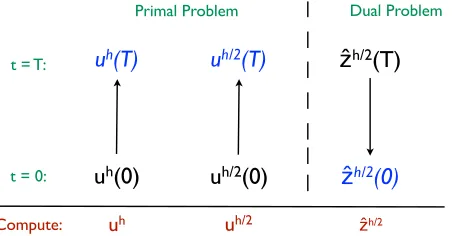
The strategy to compute ˆzh/2_{is illustrated in Figure 1. That is, the approximationsu}h

anduh/2_{are computed forward in time and subsequently ˆz}h/2 _{is obtained with a backward} in time computation.

Then, we define our error estimate, Est, as:

Qe,e(T)(u) Qe,e(T)(uh) =|||u uh|||2⇡Est:=

Z T

0 R

t _uh_{; ˆz}h/2 _dt+R0 _uh_{; ˆz}h/2 ₍₁₄₎

with the residuals_Rt_{(·;·) and R}0_{(·;·) defined in (9).}

Note that, we simply replacedze,e(T) in (12) by a computable approximation.

Remark 2.6 We approximate both the primal u and the dualz using a finer mesh than

uh_{. Thus, our estimate (14) is calculated with approximations on two di↵erent meshes,}

which motivates us to refer this procedure asduality-based two-level error estimation. _⇤

The exact error is equal to the sum of the estimate in (14) and the remainder terms due to linearization, primal approximation and dual discretization errors. We shall prove that aforementioned remainders are indeed small in the following theorem:

Theorem 2.B Let e= u uh _{and e}h/2_{:= u u}h/2 _{for any given u}h _anduh/2_{. Then for} the two-level secant dual solutionzˆdefined by (13), the following identity holds:

|||e_|||2=

Z T

0 R

t _uh_{; ˆz dt+R}0 _uh_{; ˆz + 2(((e}h/2_{, e)))}

E |||eh/2|||2. (15)

Furthermore, for the approximationzˆh/2 _{ofzˆ, we get the following equation:}

|||e_|||2=Est+r1+r2, (16)

withEst according to (14), and the remainders:

r1:= 2(((eh/2, e)))E |||eh/2|||2,

r2:=

Z T

0 R

t _uh_{; ˆz zˆ}h/2 _dt+R0 _uh_{; ˆz zˆ}h/2 _, (17)

where(((·,·)))E is the inner product associated with ||| · |||2. ⇤

Remark 2.7 The remainders are such that r1 is due to mean value linearization between

uh/2 _{and u}h _{instead of u and u}h _{and primal problem approximation replacing u by u}h/2_; andr2is due to dual problem approximation. The representations in (15) and (16) appear to be the first results which combine dual-based error representations for norms with two

Remark 2.8 The result in Theorem 2.B is dependent onC(u) being Gˆateaux (or Fr´echet)

di↵erentiable, so that the secant form in (13). _⇤

Remark 2.9 zˆh/2_{is computed backward in time on a finer mesh using (13), than as used} to computeuh_{. If the dual approximation is computed on the same mesh asu}h_{, i.e. z}h_{, one}

would obtain a useless (unreliable) estimate from the residual computation due to Galerkin

orthogonality [3]. _⇤

Remark 2.10 If the cost of computing uh/2 _{is considered excessive, higher-order} recon-struction can be used to obtain a finer primal approximation; see for instance [6]. _⇤

Proof (Proof of Theorem 2.B) Starting with (12), adding and subtractingQe,ˆˆe(T)(ˆe), and

then invoking (8), gives

|||e_|||2=Qe,e(T)(e) =

Z T

0 R

t _uh_{;z dt+R}0 _uh_{;z +Q}

ˆ

e,eˆ(T)(ˆe) Qe,ˆˆe(T)(ˆe)

=

Z T

0

Rt _uh_{;z dt+R}0 _uh_;z

+

Z T

0 R

t _uh_{; ˆz dt+R}0 _uh_{; ˆz}

Z T

0 R

t _uh_{; ˆz dt R}0 _uh_{; ˆz}

Then due to semi-linear property of Rt_{(·;·) and R}0_{(·;·), we get}

|||e|||2=Qe,e(T)(e) =

Z T

0 R

t _uh_{; ˆz dt+R}0 _uh_{; ˆz +}

Z T

0 R

t _uh_{;z z dtˆ +R}0 _uh_{;z z .ˆ}

Following from the equation above, we employ (12) again foreand ˆe:

|||e|||2=

Z T

0

Rt _uh_{; ˆz dt+R}0 _uh_{; ˆz +Q}

e,e(T)(e) Qe,ˆeˆ(T)(ˆe) (18)

The last two terms of (18) can be extended in terms of inner products:

Qe,e(T)(e) Qe,ˆˆe(T)(ˆe) =|||e|||2 |||eˆ|||2= (((e ˆe, e+ ˆe)))E. (19)

Next, writinge, eh/2 _{and ˆe in (19) in terms ofu, u}h _anduh/2_{, adding and subtracting uin} the inner product and using linearity of inner product gives

Qe,e(T)(e) Qˆe,ˆe(T)(ˆe) = (((u uh/2, u 2uh+uh/2+u u)))E

= (((eh/2,2e eh/2)))E

= 2(((eh/2, e)))E |||eh/2|||2,

which proves (15).

We need the approximate dual ˆzh/2 _{to obtain (16). By adding and subtracting the} termsR₀T_Rt _uh_{; ˆz}h/2 _{dtand R}0 _uh_{; ˆz}h/2 _{to (15), we get:}

|||e_|||2=

Z T

0 R

t _uh_{; ˆz}h/2 _dt+

R0 uh; ˆzh/2 + 2(((eh/2, e)))E |||eh/2|||2

+

Z T

0

Rt _uh_{; ˆz zˆ}h/2 _dt+R0 _uh_{; ˆz zˆ}h/2

=Est+ 2(((eh/2_{, e)))}

E |||eh/2|||2+

Z T

0 R

t _uh_{; ˆz zˆ}h/2 _dt+R0 _uh_{; ˆz zˆ}h/2 _.

⌅

3

Applications

In this section, we will consider heat and Cahn–Hilliard equations representative of a linear and nonlinear application, respectively.

3.1

Heat Equation

We chooseBu= ₄u, whereBsym_{u=BuandC(u) = 0 in the general abstract form (1)}

and obtain the following heat equation:

@tu 4u=f in ⌦T

u(0) =u0 in ⌦

u= 0 on@⌦T,

(21)

The weak form of (21) is defined by substituting the self-adjoint linear and nonlinear terms,BuandC(u), respectively in (2) and by choosing the function spaces asV =H1_(⌦),

V0_=H 1_{(⌦), so V :=L}2_{(0, T;H}1_{(⌦)), V}0_:=L2_{(0, T;H} 1_(⌦)). Using (4) withBsym_{(u, v) =}R

⌦ru·rv, we have the energy norm:

|||u_|||2_E =

Z T

0 kr

u_k2_dt+ku(T)k2_.

The semi-discrete primal problem can be written as: 1

1_{For conciseness, we present the weak formulations in Section 3 in their equivalent time–dependent}

Finduh_(t)2Vh_:

h@tuh, vi+ (ruh,rv) =hf, vi, 8v2Vh,a.e.t

uh(0) =⇡Vhu₀

(22)

Here,Vh_{is a discrete subset ofV consisting of e.g. continuous finite element functions on}

a predefined mesh and⇡Vh is the L₂-projection of u₀ ontoVh.

Following (6) and (13), the weak dual form gives: Findz 2We(T)_:

h@tz, wi+ (rz,rw) = (re,rw), 8w2V,a.e. t

z(T) =e(T), (23)

wheree =u uh _{with ¯q= e(T),q =e. In (23), all of the terms on the left hand side are}

independent of u, uh_{, since the heat equation is linear. Thus z}

e,e(T) = ˆzˆe,ˆe(T) in the case that uis replaced by uh/2 _{on the right-hand-side.}

Corollary 3.1 For approximations to the heat equation (21), the error satisfies the rep-resentation (15) in Theorem 2.B, with zˆ, the solution of (23) whereu is replaced byuh/2_. Next let the approximationzˆh/2_2Vh/2 _{be defined by:}

h @tzˆh/2, wi+ (rzˆh/2,rw) = r uh/2 uh ,rw ,8w 2Vh/2,a.e. t (24) with initial conditionzˆh/2_{(T) = u}h/2 _uh _(T).

Then, the computable estimate reduces to

Est=

Z T

0 R

t _uh_{; ˆz}h/2 _dt+

R0 uh; ˆzh/2 (25)

with (21):

Rt uh; ˆzh/2 =_hf,zˆh/2_i (_ruh,_rzˆh/2) _h@tuh,zˆh/2i

R0 _uh_{; ˆz}h/2 ₌⇣_uh/2

0 uh0; ˆzh/2(0)

⌘ (26)

for which it holds that

|||e_|||2=Est+r1+r2. (27) In particular,r1 and r2 are given explicitly in Theorem 2.B. ⇤

Proof The error satisfies (15) by the first part of the proof of Theorem 2.B for which we use the approximationuh_{and the solution ˆzfor the heat equation. (25) is introduced in the}

3.2

The Convective Cahn–Hilliard Equation

Next we consider the convective Cahn–Hilliard equation, in a convex domain⌦by choosing

Bu = r·(vu) +_{P e}"24(4u), with Bsym ₌ "2

P e4(4u) and C(u) =

1

P e4 0(u), where v is

a given smooth velocity field, satisfying divv= 0, P e is the P´ecletnumber and " is the interface thickness parameter. (u) is the nonlinear (bulk) free-energy density function, which is aC2_{-continuous, double well potential function. A common choice which we adopt} is:

(u) := 1 4 u

2 ₁ 2_.

The equation then becomes

@tu+r·(vu) +

1

P e4 "

2

4u 0(u) = 0 in⌦T

u(0) =u0 in ⌦

@nu= 0 on @⌦T

@n "24u 0(u) = 0 on @⌦T

(28)

The choices Bu and C(u) lead to a fourth-order nonlinear parabolic equation, for which we define the function spaces as _V := L2_{(0, T;H}2_{(⌦)) and V}0 _{:= L}2_{(0, T;H}2_(⌦)0_{), with}

V =H2_{(⌦) and V}0_=H2_(⌦)0_.

The corresponding energy norm from (4) withBsym_{(u, v) =}R

⌦

"2

P e4u·4v:

|||u_|||2_E :=

Z T

0

"2

P ek4uk

2_dt+ku(T)k2

The semi-discrete problem can be defined as: Finduh_(t)2Vh_:

h@tuh, vi+ (vruh, v) +

1

P e

⇣

"2 4uh,4v + (r 0_(uh_),rv)⌘_{= 0, 8v2V}h_{, a.e.t}

uh(0) =⇡Vhu₀,

(29)

where⇡_Vhu₀an L₂-projection ofu₀onto discrete space Vh. Here, V =H2(⌦) andVh is a

subset ofV consisting of, e.g. two times di↵erentiable shape functions. Then employing (6) withCs_{(u, u}h_{;w, z) =}R

⌦

1

P e4 0

s_{(u, u}h_{)wz d⌦gives the weak dual}

of (28) as:

Findz _2We(T)_:

h @tz, wi (vrz, w)+

1

P e

⇣

"24z,4w + r 0s_{(u, u}h_)z,rw ⌘₌

✓

"2

P e4e,4w

◆

for all w 2 V almost every t with ”initial’” condition z(T) = e(T), where Weu_(T)

=

v_2V,@tv2V0 :=L2(0, T;H 1(⌦)) :v(T) =u(T) uh(T) .

0s_{(u, u}h_{) is the mean-value linearization of} 0_{(u) such that:}

0s_{(u, u}h_{) =}

Z 1

0

00 _{su+ (1 s)u}h _ds=u2_{+ (u}h₎2_+uuh _1.

The right hand side of (30) shows that the dual problem is driven bye=u uh_{, while the}

left hand side shows the dependence onu, uh_{due to the nonlinear term.}

Corollary 3.2 The error in the energy-norm for the convective Cahn–Hilliard equation satisfies (15) in Theorem 2.B with uh_{, solution of (29) and zˆ, solution of (30) for u is} replaced byuh/2_{. Let also the approximationzˆ}h/2_(t)2Vh/2 _{be defined by:}

h @tzˆh/2, wi vrzˆh/2, w +

1

P e

⇣

"2_4ˆzh/2_{,4w + r} 0s_(uh/2_{, u}h_)ˆzh/2_,rw ⌘

=

✓

"2

P e4(u

h/2 _uh_),

4w

◆

,

(31)

8w₂Vh/2 _{almost every t, with ”initial” conditionzˆ}h/2_{(T) = u}h/2 _uh _(T). The computable estimate then becomes

Est=

Z T

0 R

t _uh_{; ˆz}h/2 _dt+R0 _uh_{; ˆz}h/2 ₍₃₂₎

where

Rt _uh_{; ˆz}h/2 _{= h@}

tuh,zˆh/2i (vruh,zˆh/2)

1

P e

⇣

"2(4uh,4zˆh/2) (r 0_(uh_),rzˆh/2₎⌘

R0 _uh_{; ˆz}h/2 ₌⇣_uh/2

0 uh0(0),zˆh/2(0)

⌘

,

(33)

for which it holds that:

|||e_|||2=Est+r1+r2 (34)

withr1and r2 introduced in Theorem 2.B. ⇤

Proof The error satisfies (15) by employing the first part of the proof in Theorem 2.B with uh _{and ˆz of Cahn–Hilliard equation. The computable estimate (32) is in the same}

form as (14), for which the residuals in (33) are computed using approximationuh _{in (29)}

and approximation ˆzh/2_{in (31). Then (34) is straightforward result of Theorem 2.B.}

Computing the approximate solutionsuh_{, u}h/2 _{and z}h/2 _{need higher-order discrete spaces} withC1_{-continuity. These have been pursued in [20] and [37]. In order to avoid the direct} spatial discretization of a fourth-order operator in numerical computations, we continue in the next section with the Cahn–Hilliard equation in a mixed formulation as two second-order equations.

3.2.1 Mixed Formulation of the Convective Cahn–Hilliard Equation

In the mixed formulation, a new variableµ, called chemical potential is introduced. The the set of equations becomes

@tu+r·(vu)

1

P e4µ= 0 in⌦T µ 0(u) +"24u= 0 in⌦T

u(0) =u0 in ⌦

@nu=@nµ= 0 on @⌦T.

(35)

System (35) does not immediately fit the general form in (2). Nevertheless, the general setting can be straightforwardly extended to account for systems.

We will set the corresponding energy norm as:

|||(u, µ)|||2

E :=

Z T

0

✓

"2kruk2₊ 1

P ekrµk

2

◆

dt+ku(T)k2_{. (36)}

The weak form of (35) becomes: Find (u, µ)2Wu0⇥V

hut, vi+ (vru, v) +

1

P e(rµ,rv) = 0, 8v2V

(µ, w) ( 0(u), w) "2(_ru,_rw) = 0, ₈w₂V,

(37)

where _V = L2_{(0, T;H}1_{(⌦)) and W}

u0 = {v2V,@tv2V0:=L

2_{(0, T;H} 1_{(⌦)) :v(0) =u0}} The semi-discrete weak form of (35) is:

Finduh_{(t), µ}h_(t)2Vh

h@tuh, vi+ vruh, v +

1

P e rµ

h_{,rv = 0, 8v2V}h

µh, w 0(uh), w "2 ruh,rw = 0, 8w2Vh uh(0) =⇡Vhu₀,

(38)

The weak dual system of mixed formulation is (see [39]): Find (z, )_2Weu_(T)

⇥V:

h @tz,⌫i (vrz,⌫) "2(r ,r⌫) 0s(u, uh) ,⌫ = "2(reu,r⌫)

( ,⌘) + 1

P e(rz,r⌘) =

1

P e(re

µ_,

r⌘)

z(T) =eu(T)

(39)

for almost everytand for all ⌫,⌘2V, where (z, ) is the dual pair of (u, µ) and 0s_{(u, u}h₎

is the mean-value linearization of 0(u) as in Section 3.2.

The right hand side of (39) shows that the dual problem is driven by the ap-proximation error in u and µ, which are eu _{:= u u}h _{and e}µ _{:= µ µ}h_,

while the term 0s_{(u, u}h_{) on the left hand side is dependent on u and u}h _due

to linearization. Furthermore, the dual space for z can be defined as Weu_(T)

=

v_2V,@tv2V0 :=L2(0, T;H 1(⌦)) :v(T) =eu(T)=u(T) uh(T)

Proposition 3.3 Let (ˆz,ˆ) be the solution pair of (39) for uand µare replaced by uh/2 and µh/2_{, respectively. Then the error measure for mixed formulation of Cahn–Hilliard} equation satisfies:

|||(eu, eµ)|||2₌

Z T

0

⇣

Rt

1 uh; ˆz +Rt2 µh; ˆ

⌘

dt+R0 _uh_{; ˆz}

+ 2((( (euh/2, eµh/2),(eu, eµ) )))E |||(eu

h/2

, eµh/2)|||2_,

(40)

where eu _{= u u}h_{, e}µ _{= µ µ}h _{and e}uh/2

= u uh/2_{, e}µh/2

= µ µh/2 _{for any given}

uh_{, u}h/2_{, µ}h _andµh/2_.

Furthermore, for zˆh/2_,ˆh/2 _{of (ˆz,ˆ), we get:}

|||(eu, eµ)|||2_=Est+r

1+r2, (41)

where Est= Z T 0 ⇣ Rt

1 uh; ˆzh/2 +Rt2 µh; ˆh/2

⌘

dt+R0 _uh_{; ˆz}h/2 ₍₄₂₎

with residuals

Rt

1 uh; ˆzh/2 = h@tuh,zˆh/2i (vruh,zˆh/2)

1

P e(rµ

h_,rzˆh/2₎

Rt

2 µh; ˆh/2 = (µh,ˆh/2) + ( 0(uh),ˆh/2) +"2(ruh,rˆh/2) R0 _uh_{; ˆz}h/2 ₌⇣_uh/2

0 uh0,zˆh/2(0)

⌘

.

and the remainders

r1:= 2((( (eu

h/2

, eµh/2),(eu, eµ) )))E |||(eu

h/2

, eµh/2)_|||2,

r2:=

Z T

0

⇣

Rt

1 uh; ˆz zˆh/2 +Rt2 µh; ˆ ˆh/2

⌘

dt+_R0 _uh_{; ˆz zˆ}h/2 _. (44)

⇤

Proof We can not apply Theorem 2.B, but we closely follow its proof. Using (36), the error writes:

|||(eu, eµ)_|||2=Qeu_,eµ_,eu_(T)(eu, eµ) =

Z T

0

✓

"2

P ekre

u

k2+ 1

P ekre

µ

k2

◆

dt+_ku(T)_k2

=

Z T

0

⇣

Rt

1 uh;z +Rt2 µh;

⌘

dt+R0 _uh_;z

Then by adding and subtractingQeˆu_,ˆeµ_,eˆu_(T)(ˆeu,eˆµ) with ˆeu:=uh/2 uhand ˆeµ:=µh/2 µh

and due to semi-linearity of_R, the error representation becomes:

|||(eu_{, e}µ_)|||2 ₌

Z T

0

⇣

Rt

1 uh;z +Rt2 µh;

⌘

dt+_R0 _uh_{;z +Q}

ˆ

eu_,eˆµ_,ˆeu_(T)(ˆeu,eˆµ)

Qeˆu_,eˆµ_,ˆeu_(T)(ˆeu,eˆµ)

=

Z T

0

⇣

Rt1 uh; ˆz +Rt2 µh; ˆ

⌘

dt+_R0 uh; ˆz

+

Z T

0

⇣

Rt

1 uh;z zˆ +Rt2 µh; ˆ

⌘

dt+R0 _uh_{;z zˆ}

=

Z T

0

⇣

Rt

1 uh; ˆz +Rt2 µh; ˆ

⌘

dt+_R0 _uh_{; ˆz +Q}

eu_,eµ_,eu_(T)(eu, eµ)

Qeˆu_,eˆµ_,ˆeu_(T)(ˆeu,eˆµ) (45)

We can extend the last two terms in (45) in terms of inner products and write the errors in terms ofu, uh_{, u}h/2 _{andµ, µ}h_{, µ}h/2_.

Qeu_,eµ_,eu_(T)(eu, eµ) Q_eˆu_,ˆeµ_,ˆeu_(T)(ˆeu,eˆµ) =|||(eu, eµ)|||2 |||(ˆeu,eˆµ)|||2

Then using linearity of the inner product after adding and subtracting u and µ to the second part of the product gives

|||(eu, eµ)|||2 _{||| e}uˆ_{, e}µˆ _|||2_{= ((( (e}u_{, e}µ_{) (ˆe}u_,eˆµ_),(eu_{, e}µ_{) + (ˆe}u_,ˆeµ_{) )))} E

= (((u uh/2+µ µh/2, u 2uh+µ 2µh+uh/2+µh/2

+u u+µ µ)))E

= ((( (euh/2

, eµh/2

),2(eu_{, e}µ_{) (e}uh/2

, eµh/2

) )))E

= 2((( (euh/2, eµh/2),(eu, eµ) )))E |||(eu

h/2

which proves (40).

Next, if we add and subtract the terms R₀T⇣_Rt

1 uh; ˆzh/2 + Rt2 µh; ˆh/2

⌘

dt + R0 _uh_{; ˆz}h/2 _{from (40), we obtain (41) such that}

|||(eu, eµ)_|||2=

Z T

0

⇣

Rt1 uh; ˆzh/2 +Rt2 µh; ˆh/2

⌘

dt+_R0 uh; ˆzh/2

+ 2((( (euh/2, eµh/2),(eu, eµ) )))E |||(eu

h/2

, eµh/2)_|||2

+

Z T

0

⇣

Rt

1 uh; ˆz zˆh/2 +Rt2 µh; ˆ ˆh/2

⌘

dt+_R0 _uh_{; ˆz zˆ}h/2 _,

which gives the computable estimate (42). In particular, one can obtain the residuals (43)

following the proof of Theorem 2.A. _⌅

4

Numerics

In this section, the performance of the duality-based two-level estimator is illustrated for linear heat and nonlinear convective Cahn–Hilliard equations. We focus on errors due to spatial discretization.

For discretization in space, we use piecewise linear finite element approximations for the heat equation and the mixed formulation of the Cahn–Hilliard equation. For time discretization, we use the backward Euler method for the heat equation and a first-order semi-implicit splitting scheme from [18] for Cahn–Hilliard equation. Recent second-order time schemes for Cahn–Hilliard models can be found in [46, 47]. In the numerical experi-ments, the time step is chosen sufficiently small for both of the equations, in order to avoid time errors due to time discretization.

The results will be investigated in two parts: The first part, Section 4.1, is about the convergence of the estimate (14) under uniform space refinements. The second part, Section 4.2, is devoted to adaptivity. In this section we consider adaptive mesh-refinement employing the duality-based two-level error estimates.

Remark 4.1 The general estimateEstintroduced in (14) is localized in this section both in space and in time. In particular, the results presented in Section 4.1, computes Est

by localizing only in time, but global in space. However, in Section 4.2, the indicator is

4.1

Convergence and E

↵

ectivity

We test the convergence against true errors and present e↵ectivity indices for 1D and 2D test cases. E↵ectivity is the ratio of the estimator to the true error:

E↵ectivity = Est

Qe,e(T)(e)

= Est |||e_|||2.

E↵ectivity values in the range 0.1 _⇠ 10 are generally considered acceptable, however, ideally it is close to 1.

4.1.1 Heat Equation

We first consider the linear heat equation with zero Dirichlet boundary conditions. We computed heat equation for single and 100 time steps in⌦= [0,1]d _{withd2{1,2}. Here,}

heat equation is considered in the case of absence of source, that is,f = 0.

To evaluate the estimateEst, space-time approximations are required. The backward Euler scheme yields approximations uh

k, at discrete time instances. We define all

approxi-mations uh_{, u}h/2 _{and ˆz}h/2 _{using a piecewise-constant reconstruction for allt2[0, T] such} that

uh(t) =uh_k+1, t2 tk, tk+1

⇤

ˆ

zh/2(t) = ˆz_kh/₊₁2, t₂⇥tk, tk+1

fork = 0, . . . , N 1, then (25) becomes2

Est=

N 1

X

k=0

⇢

t⇣hfk+1,zˆkh/2i (ruhk+1,rzˆ

h/2

k )

⌘

(uh_k+1 uh_k,zˆ_kh/2) . (46)

We can compute part of the estimate at each time step and sum up to the final time,T.

1D Simulation We take the initial data as:

u(x,0) = sin(⇡x), x₂[0,1]

2_{One can not immediately substitute piecewise-constant reconstruction in the representation formula}

(25) because ofut. To obtain the result (46), one can use a limiting procedure on a continuous piecewise

linear function. For example, use the following reconstruction

uh_{(t) =}

( _{uk+1 uk}

tk+✏ tk (t tk+✏) +uk+1 fortk< ttk+✏;

uk+1 fortk+✏< ttk+1.

and computeuh_2Vh _{with 2}3_,24_{, . . . ,2}9 _{elements, i.e. h= 2} 3_,2 4_{, . . . ,2} 9_{. We use time} step size t = 0.0005. The overkill solution for the exact error is computed using 213 elements. To compute the dual, we use a uniformly refined space Vh/2 _{with 2}4_{, . . . ,2}10 elements. We also investigate the use of a better, but two times more expensive spaceVh/4 instead ofVh/2 _{with 2}5_{, . . . ,2}11_elements.

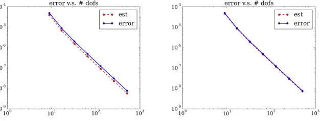
Figure 2: Convergence of error and estimateEst with respect to uniform refinement for single time step with two levelsVh_andVh/2_(left),andVh _andVh/4 _{(right) for heat equation in 1D.}

We choose q = u uh _{and ¯q = u(T) u}h_{(T) as in (23) and to compute the dual}

approximation, u is replaced with the approximations in Vh/2 _{and V}h/4_{. In Figure 2, we} see that the estimate asymptotically bounds the error up to a constant which confirms the e↵ectivity of the two-level estimate.

Nb of Elems E↵(uh_{; ˆz}h/2_{) E↵ (u}h_{; ˆz}h/4₎

16 0.77210875 0.94439973

32 0.75602279 0.93939171

64 0.75158218 0.93803695

128 0.75056921 0.93784922

256 0.75082958 0.93844620

Table 1: E↵ectivity of single time step estimate for heat equation in 1D.

In Table 1, the e↵ectivity indices are displayed for the dual approximations computed in the two di↵erent discrete spaces (i.e. Vh/2 _{and V}h/4_{). The accuracy of the estimate} increases when ˆzh/4 _{is used instead of ˆz}h/2 _{to compute Est.}

Figure 3: Convergence of error and estimateEstwith respect to uniform refinement for 100 time steps with two levelsVh_andVh/2_(left),andVh_andVh/4_{(right) for heat equation in 1D.}

(uh_{; ˆz}h/2_{) (u}h_{; ˆz}h/4₎

Nb of Elems Est E↵ Est E↵ Qe,e(T)(e)

16 3.6257e-04 0.7206 4.5308e-04 0.9005 5.0311e-04 32 9.0464e-05 0.7205 1.1307e-04 0.9006 1.2554e-04 64 2.2605e-05 0.7205 2.8255e-05 0.9007 3.1369e-05 128 5.6505e-06 0.7207 7.0631e-06 0.9009 7.8400e-06 256 1.4125e-06 0.7212 1.7657e-06 0.9015 1.9585e-06

Table 2: Estimate, error and e↵ectivity for 100 time steps for heat equation in 1D.

ˆ

z computed in spaces Vh/2 _{and V}h/4 _{with respect to uniform refinement. The e↵ectivity} index is⇠0.7 when we use ˆzh/2 _{to compute estimate, whereas it increases to⇠0.9 with} ˆ

zh/4_.

We observe that the additional cost of the computation is significant using the more expensive space Vh/4_{, however, the e↵ectivity constants are still acceptable for the space}

Vh/2_{. Therefore, for the rest of the paperV}h_{and V}h/2 _{spaces will be used for the sake of} computational cost.

2D Simulation Next, we ran the simulation in 2D with time step size of t = 0.0005 using the following initial condition

u(x, y,0) = sin(⇡x) sin(⇡y).

Figure 4: Convergence of error and estimate Est with respect to uniform refinement for single time step with two levelsVh_andVh/2

for heat equation in 2D.

(uh_{; ˆz}h/2₎

Nb of Elems Est Qe,e(T)(e) E↵

42 _{3.8028e-04 4.2845e-04 0.8875} 82 _{3.9390e-05 4.8174e-05 0.8176} 162 _{6.806e-06 8.7837e-06 0.7748} 322 _{1.5180e-06 1.9775e-06 0.7676} 642 _{3.6813e-07 4.5946e-07 0.8012}

Table 3: Estimate, error and e↵ectivity for single time step for heat equation in 2D.

Figure 5: Convergence of error and estimate Est with respect to uniform refinement for 100 time steps with two levelsVh_andVh/2

for heat equation in 2D.

(uh_{; ˆz}h/2₎

Nb of Elems Est Qe,e(T)(e) E↵ 42 _{3.6420e-03 5.7110e-03 0.6377} 82 _{8.8885e-04 1.3861e-03 0.6412} 162 _{2.2091e-04 3.4304e-04 0.6439} 322 _{5.5148e-05 8.4601e-05 0.6518} 642 _{1.3782e-05 2.0134e-05 0.6845}

Table 4: Estimate, error and e↵ectivity for 100 time steps with two levelsVh_{and V}h/2 _{for heat}

equation in 2D.

In Figure 4 and 3, we present the convergence of estimate and the error with e↵ectivity indices for one time step in 2D. The plot (left) shows that the estimate bounds the error asymptotically up to a constant which is presented in the table (right). Th e↵ectivity index in ⇠0.8, which shows the estimate is e↵ective.

is⇠0.6.

4.1.2 The Convective Cahn–Hilliard Equation

Next, the convective Cahn–Hilliard Equation is considered in mixed formulation, see Sec-tion 3.2.1. Since the Cahn–Hilliard equaSec-tion is a nonlinear phase-field model, the estimaSec-tion of errors can be illustrated with two test cases: Moving interface and merging two bubbles close to each other.

Similar to the heat equation approximation in Section 4.1.1, we define space-time pri-mal and dual approximations with piecewise-constant reconstruction for the semi-implicit scheme applied to Galerkin finite element discretization of the mixed formulation. The reconstructions are:

uh(t) =uh_k+1 andµh(t) =µh_k+1, t₂ tk, tk+1

⇤

ˆ

zh/2_{(t) = ˆz}h/2

k+1 and ˆh/2(t) = ˆ

h/2

k+1, t2

⇥

tk, tk+1

fork = 0, . . . , N 1. Then we can write estimate (42) as 3

Est=

N_X1

k=0

⇢

t⇣ (v_ruh_k+1,zˆ_kh/2) 1

P e(rµ

h k+1,rzˆ

h/2

k ) (µ h k+1,ˆ

h/2

k )

+ ( 0(uh k+1), ˆ

h/2

k ) +"2(ruhk+1,rˆ

h/2

k )

⌘

(uh

k+1 uhk,zˆ h/2

k ) .

(47)

The discrete estimate (47) can be computed at each time step and summed up for the final time,T.

For the simulation of the Cahn–Hilliard equation, we choose q1 = "2eu, q2 = eµ and ¯

q=e(T) as in (39) and we take "= 0.0625 and P e= 1.

Moving Interface We simulate the moving interface test case for 1D and 2D and we set the domain ⌦= [0,1]d_{, for d2{1,2}. In 1D, we impose an initial condition for u}

0as:

u(x,0) = tanh

✓

x 0.25 p

2"

◆

, x₂[0,1] (48)

and we takev= 0.05 for which the solution propagates as a front to the right.

3_{as in the heat equation case the piecewise-constant reconstruction can not be substituted immediately.}

We compute Est with uh_{, µ}h _2Vh _{and ˆz}h/2_,ˆh/2 _{2 V}h/2_{, for which we use 2}3_{, . . . ,2}9 and 24_{, . . . ,2}10 _{elements, respectively. For the overkill solution, we use 2}13 _{elements. In} order to obtain higher e↵ectivity, we also choose two times refined space thanVh_{, which}

isVh/4 _{with 2}5_{, . . . ,2}11 _elements.

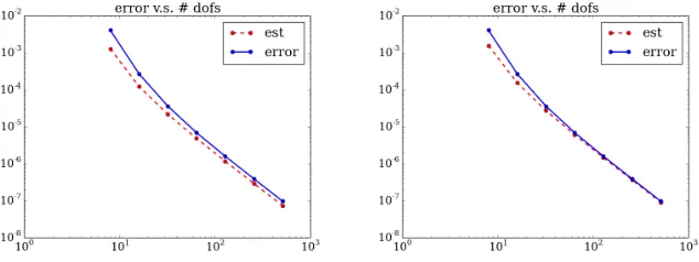
Figure 6: Convergence of error and estimateEstwith respect to uniform refinement for 100 time steps with two levels Vh _{and V}h/2 _{(left), and V}h _{and V}h/4 _{(right) for Cahn–Hilliard equation,}

moving interface test case in 1D.

(uh_{, µ}h_{; ˆz}h/2_,ˆh/2_{) (u}h_{, µ}h_{; ˆz}h/4_,ˆh/4₎

Nb of Elems Est E↵ Est E↵ Qeu_,eµ_,eu_(T)(e)

16 1.2205e-04 0.4559 1.5419e-04 0.5760 2.6772e-04 32 2.1533e-05 0.6002 2.7088e-05 0.7550 3.5876e-05 64 4.8082e-06 0.6987 6.0224e-06 0.8751 6.8813e-06 128 1.1656e-06 0.7350 1.4578e-06 0.9193 1.5857e-06 256 2.8913e-07 0.7457 3.6146e-07 0.9323 3.8771e-07

Table 5: E↵ectivity of 100 time steps estimate for Cahn–Hilliard equation, moving interface test case in 1D.

We present the convergence plots in Figure 6 for 100 time steps in 1D with t= 0.0005. One can observe that the estimate bounds the error asymptotically up to a constant for both plots. The estimate gets closer to the error when (ˆzh/4_,ˆh/4_{) is used instead of} (ˆzh/2_,ˆh/2_).

Similarly, Table 5 enables a fair comparison of error, estimate and e↵ectivity. E↵ectivity index increases, if the computation is done using the pair (ˆzh/4_,ˆh/4_{) instead of (ˆz}h/2_,ˆh/2_).

We also ran the simulation in 2D and use the initial condition

u(x, y,0) = tanh

✓

x 0.25 p

2"

◆

with v = (0.05,0). uh_{, µ}h _{2 V}h _{are computed with 2}2_⇥22_{, . . . ,2}6_⇥26 _{elements and for} the dual pair ˆzh/2_,ˆh/2_2Vh/2 _{we use 2}3_⇥23_{, . . . ,2}7_⇥27 _{elements. The overkill solution} is computed with 28_⇥28 _elements.

Figure 7: Convergence of errror and estimateEst with respect to uniform refinement for 1 (left) and 100 (right) time steps with two levels Vh _{and V}h/2 _{for Cahn–Hilliard equation, moving}

interface test case in 2D.

T = 0.0005 T = 0.05

Nb of Elems Est Qeu_,eµ_,eu_(T)(e) E↵ Est Q_eu_,eµ_,eu_(T)(e) E↵

42 _{1.9926e-02 2.5232e-02 0.7897 9.9011e-03 3.6916e-02 0.2682} 82 _{1.4882e-03 2.1692e-03 0.6860 1.2766e-03 4.0469e-03 0.3154} 162 _{5.0831e-05 7.4457e-05 0.6827 1.2204e-04 2.6622e-04 0.4584} 322 _{3.0019e-06 4.3608e-06 0.6883 2.1531e-05 3.5200e-05 0.6116} 642 _{2.2099e-07 3.0101e-07 0.7342 4.8088e-06 6.4280e-06 0.7481}

Table 6: E↵ectivity of 1 and 100 time steps estimate for Cahn–Hilliard equation, moving interface test case in 2D.

In Figure 7 and Table 6, 1 and 100 time steps results are considered. In both of the plots of Figure 7 we observe the convergence behavior such that the error is bounded below asymptotically. In the pre-asymptotics, we can see from left plot of Figure 7 that the error and the estimate are converging with the same order for 1 time step. For 100 time step, they start with a low convergence rate, then estimate gets closer to the error as the number of dofs increase. This is also confirmed by the e↵ectivity indices in Table 6.

Remark 4.2 We also test the two-level estimator based on a linear quantity of interest:

Q(u) :=

Z

⌦

sin(⇡x)u(T)d⌦, (50)

which is obtained by choosingq= 0 and ¯q= sin(⇡x) in (5), for which the estimate is again of the same form as in (47).

The results presented in Figure 8 and Table 7 are obtained for the moving interface test case of 1D Cahn–Hilliard equation for 100 time steps with t= 0.00001 under uniform re-finement, and confirm the expected consistency of the estimator. The convergence behavior slightly deviates because of errors due to time discretization (not taken into account).

Figure 8: Convergence of error and estimate Est with respect to uniform refinement for 100 time steps with two levelsVh_andVh/2

for Cahn–Hilliard equation, moving inter-face test case in 1D and forQ(_·) in (50).

(uh_{, µ}h_{; ˆz}h/2_,ˆh/2₎

Nb of Elems Est Qe,1(e) E↵

16 2.5443e-05 2.7887e-05 0.9123 32 4.8486e-06 6.1084e-06 0.7937 64 1.1236e-06 1.4727e-06 0.7629 128 2.8921e-07 3.6475e-07 0.7929 256 8.4079e-08 9.0913e-08 0.9248

Table 7: Estimate error and e↵ectivity for 100 time steps with two levelsVh_andVh/2_{for Cahn–}

Hilliard equation, moving interface test case in 1D and forQ(_·) in (50).

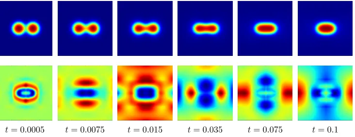
Merging Bubble in 2D The final numerical experiment is the case of two bubbles merging. We consider the error measure of (36) by aiming to estimate the error particularly for the physics of a topological change. We take the Cahn–Hilliard equation without convection, i.e., v = 0 and take the following initial condition corresponding to kissing bubbles of the same radius, 0.2 in⌦= [0,1]⇥[0,1] :

u(x,0) = 1 + tanh 0.2

p

(x 0.25)2_+y2 p

2"

!

+ tanh 0.2

p

(x+ 0.25)2_+y2 p

2"

!

.

We present 2D results with time step size, t= 0.0005 for 200 time steps. In Figure 9, the solution of the merging case can be seen.

t= 0.0005 t= 0.0075 t= 0.015 t= 0.035 t= 0.075 t= 0.1

Figure 9: Two merging bubbles in 2D: primal,u(top), dual (bottom)

Figure 10: Convergence of error and esti-mate Est with respect to uniform refine-ment for 200 time steps with two levelsVh andVh/2_{for Cahn–Hilliard equation,}

merg-ing bubble test case in 2D.

(uh_{, µ}h_{; ˆz}h/2_,ˆh/2₎ Nb of Elems Est Qe,e(T)(e) E↵

42 _{1.5969e-02 1.6640e-01 0.0959} 82 _{1.0217e-02 4.9134e-02 0.2079} 162 _{2.4790e-03 1.0568e-03 0.2345} 322 _{5.3838e-04 1.7559e-03 0.3066} 642 _{1.2160e-04 2.9331e-4 0.4145}

Figure 11: Estimate, error and e↵ectivity for 200 time steps with two levelsVh_andVh/2_{for Cahn–}

Hilliard equation, merging bubble test case in 2D.

Remark 4.3 (Direct error estimation) For a merging bubble test case in 1D, Figure 12 shows a comparison of time-contributions to the two-level estima-tor (blue curve) and the direct space-time error estimator _||uh/2 _uh_||2 _:=

RT

0 "

2_{kr u}h/2 _uh _k2₊ 1

P ekr µ

Figure 12: Comparison of time-contributions to Est and _kuh/2 _uh_k2_.

4.2

Adaptivity

We now consider adaptivity based on the indicators, which contain not only the information for the current time step but also the whole evolution history implicitly via the dual. The proposed global-time space-adaptive algorithm for our error measure (8) is presented in Algorithm 1.

The numerical test cases we provide later are preliminary adaptive tests aimed at demonstrating how the new estimator can be employed in the adaptive strategy. And for the sake of simplification, we only consider adaptivity in space.

We note that adaptivity for time-dependent problems has additional overhead in its numerical implementation, such as projection / interpolation between meshes, and multiple space-time solves. However, the advantage of adaptivity is clear: one obtains optimized meshes at each time instance for the solution at hand.

The computable estimator (14) is a global space-time residual weighted with the dual approximation. Assuming piecewise-constant reconstruction of the primal solution and the dual solution, the estimator splits up as,

Est=

N_X1

k=0

⇣

tRt_(uh k+1; ˆz

h/2

k ) + (uhk uhk+1,zˆ

h/2

k )

⌘



N_X1

k=0

Estk (51)

where

Estk := tRt(uhk+1; ˆz

h/2

k ) + (uhk uhk+1,zˆ

h/2

k ). (52)

Algorithm 1 The global-time space-adaptive algorithm

Choose an initial coarse mesh _K and a small enough time step size t

Initialize a list of mesh{K1, ...,KN}, one individual mesh for one time step

whilethe maximal error estimate M AX >tolerance do for every time stepk (t:= 0_!T)do

Compute the primal solution uh

k using the current mesh Kk

Compute the primal solutionuh/_k 2using the finer mesh_Kh/_k 2(i.e. _Kh/_k 2is the uniform refinement ofKk)

end for

for every time stepk (t:=T _!0)do

Compute the dual solution ˆz_kh/2 using the finer mesh_Kh/_k 2 Estimate the current mesh error contributionEstk

end for

Compute the maximal error contribution for the whole time period M AX = max_{Est1, ..., EstN}

while|Estk|>✓|M AX| do

Estimate the local error contribution⌘i

k for the meshKk

Refine the mesh_Kkby using hierarchical refinement strategy and maximum strategy

functions'i _2Vh/2_{, i= 1, ..., M. The dual solution can be written as the linear} combina-tion,

ˆ

z_kh/2=

M

X

i=1 ˜

z_ki'i. (53)

Inserting the ansatz (53) into (52), we get

Est=

N_X1

k=0

M

X

i=1

⇣

tz˜_ki _Rt(u_kh₊₁;'i) + ˜z_ki (uh_k uh_k+1,'i)⌘. (54)

Thus, the error estimator is localized to the basis. This is similar to the localization approach in [10]. The indicator for each basis function 'i _{in V}h/2 _{at each time step k is} thus:

⌘i

k= tz˜ki Rt(uhk+1;'i) + ˜zik uhk uhk+1,'i . (55) The same as localizing the indicator, the error control is also built on a two-step ap-proach. First, we apply the maximum marking strategy with fraction✓2[0,1] onEstk, to

select which time steps contain the big error contributions throughout the time period. To reduce the error, the corresponding space meshes at the selected time steps are targeted to be refined. Then, the maximum marking strategy is applied second time for selecting basis function inVh/2_{. The indicator of the selected basis is at least a fraction 2 [0,1]} bigger than the maximal indicator (i.e. |⌘i| max(|⌘i|)).

The mesh refinement is based on the hierarchical refinement strategy in [45, 26]. Since

Vh/2 _{is the uniform refined space of V}h_{, the parents of the basis functions inV}h/2 _{are the} basis functions inVh_{. Thus, for the selected basis inV}h/2_{, the mesh inV}h _{can be refined}

according to the parent of the basis in Vh/2_.

Remark 4.4 (Hierarchical Indicator) In general, the standard indicator for the dual weighted residual (DWR) method is obtained by applying integration by parts after lo-calizing the indicator elementwise as in [6]. In particular, for the DWR indicators, the interpolant of the dual solution, Izˆ_kh/2, is subtracted from ˆz_kh/2 to get a sharper indicator. However, for hierarchical indicators, like (55), instead of using integration by parts, the indicator is localized through patches of elements corresponding to the support of basis functions. Hence, the indicator in (55) is expected to be sharp. Let us show that (55) is equivalent to the indicator obtained by localizing the residual weighted by ˆz_kh/2 Izˆh/_k 2. Consider

⌘k= tRt

⇣

where, by Galerkin orthogonality,

t_Rt⇣_uh k+1;Izˆ

h/2

k

⌘

+⇣uh

k uhk+1, Izˆ

h/2

k

⌘

= 0.

The interpolant Izˆ_kh/2, similar to (53), can be written as a linear combination of shape functions:

Izˆ_kh/2=

M

X

i=1 ¯

z_ki'i=

M

X

i=1 ˜

z_kiI'i,

then (56) can be rewritten as

⌘k= M

X

i=1

⇣

t_Rt_(uh

k+1; ˜zki'i z¯ik'i) + (uhk uhk+1,z˜ki'i z¯ik'i)

⌘ = M X i=1 ⇣

t_Rt(uh_k+1; ˜z_ki'i z˜i_kI'i) + (uh_k uh_k+1,z˜_ki'i z˜i_kI'i)⌘.

=

M

X

i=1

⇣

tz˜i_kRt _uh

k+1; 'i I'i + ˜zki uhk uhk+1, 'i I'i

⌘

.

Hence, Galerkin orthogonality

t_Rt uh_k+1;I'i + uh_k uh_k+1, I'i = 0

implies

⌘_ki = tz˜_ki _Rt(uh_k+1;'i) + ˜z_ki uh_k uh_k+1,'i

= tz˜_ki _Rt(uh_k+1; 'i I'i ) + ˜z_ki uh_k uh_k+1, 'i I'i

which coincides with the localized indicator (55). _⇤

4.2.1 Heat Equation

We begin with verifying numerically our global-time space-adaptive algorithm with the linear heat equation (21). The dynamics of this test case is one bubble smoothed out in the middle of the domain. The initial condition is assumed to be:

u(x,0) = tanh⇣50 0.2 px2_+y2 ⌘_{+ 1 (57)}