Modeling the Signature of Sulfur Mass Independent Fractionation produced in the Archean Atmosphere

Appendices for “Modeling the Signature of Sulfur Mass-Independent Fractionation produced in the Archean Atmosphere”

Appendix I - Validation

Appendix II - Additional tests of Halevy et al. (2010)

Appendix III - Additional model results, including DA08 and the SO2 photoexcitation band

Appendix I - Validation

We followed the overall numerical methodology of Pavlov and Kasting

(2002) in our sulfur isotope calculations. Briefly, this involves assuming that minor

sulfur isotopes species do not affect the concentrations of the major (32S) species, and ignores both doubly substituted sulfur species and reactions

involving more than one isotopic substituted species. Furthermore, we adjusted

reaction rate constants to maintain mass balance in the case of self-reactions or

multiply branching pathways (Pavlov and Kasting, 2002). While we followed

existing methodology, we re-wrote the numerical code independently, so present

4 diagnostic cases to ensure reliability:

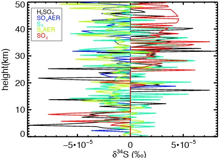
I-a Using the 32SO2 cross section in place of minor isotopes

If the 32SO2 cross-section is used in place of the 34SO2 cross-section, a

correctly functioning model should produce no fractionation. Figure A1 shows

the δ34S computed under this test, revealing fractionations at the ~5x10-5 ‰ level,

up to a maximum of 10-4 ‰ (1 part in 10-7), which is the machine limit for a FORTRAN single-precision floating-point number. All internal calculations are

0±3x10-5 ‰. Therefore, this test supports the numerical validity of our model.

Figure A1 – A calculation showing fractionations at the lower limit of calculable outputs when the 32SO2 cross-section is used for 34SO2.

I-b Modeling both mass-dependent fractionation and mass-independent

fractionation

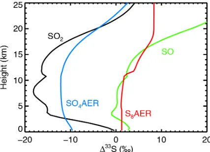
We do not include any mass-dependent fractionation processes in our

standard model, so our predicted δ33S and δ34S magnitudes only reflect the

mass-independent contributions induced by the isotopologue absorption

cross-sections. In addition, our δ33S and δ34S values are computed relative to standard

that we set to 1. Therefore our predictions for Δ33S magnitudes are

representative of those produced in the atmosphere, but the specific magnitudes

ï‡

‡

I

_{S (‰)}

height(km)

H SO

SO4AER S

S₈AER

SO₂ 2 4

of δ33S and δ34S could be changed by additional photochemical reactions and are

not directly comparable to data without re-normalization of the standard. As a

further check of our methodology, we ran the standard model with rate constants

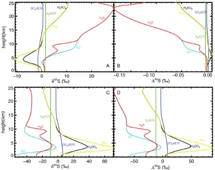
subject to dependent fractionation, both with and without the

mass-independent contributions. We chose the reaction SO + O + M → SO2 + M, for

which we arbitrarily assumed fractionation factors (=0.98) of 20 ‰ in δ34S and

10.3 ‰ (=0.9897) in δ33S. These fictitious adjustments to the reaction rate

constants yielded large δ34S (Fig A2a) but only very small mass-independent

fractionations (Fig A2b). The mass-independent fractionations imparted in the

stratosphere are of the order of 0.15‰, magnitudes that are generally

indistinguishable from mass-dependent production processes (Farquhar et al.,

2007 ; Johnston, 2011). The tropospheric MIF signatures that are likely to be

delivered to the Archean rock record from a representative atmospheric

mass-dependent processes imparting a 20 ‰ δ34S fractionation are ~0.01‰.

We next ran the standard model with both the mass-dependent

fractionation pathway as well as through the DA08 cross sections. The δ34S

fractionations from the mass-independent pathway dominate the resulting

atmospheric profile (Fig A2c), although there is obvious alteration from the δ34S

profile in the standard model. Figure A2d shows that the predicted Δ33S signal is

Figure A2 – Calculation showing mass-dependent fractionation. a/b) Models run with mass-dependent fractionation only. c/d) the standard model along with mass-dependent fractionation.

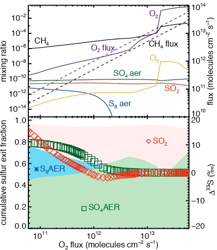
I-c Modeling a “rise of O2” scenario

Figure A3 shows a suite of model runs similar to those in Fig. 7, but

lacking any background CH4 levels. The CH4:O2 flux ratio is therefore maintained

at exactly 0.5 as the O2 flux increases from left to right, rather than ~0.6 as it was

on the right hand side of Fig. 7. In this experiment, O2 and CH4 mixing ratios

increase monotonically, but the atmosphere switches to an oxic state at an O2

to produce small MIF-S signals, with SO2 taking on negative Δ33S magnitudes (up

to ~ -1‰) while sulfate retains small positive magnitude Δ33S. As the atmosphere

becomes oxic (i.e., as the ozone layer forms (Kasting and Donahue,1980; Claire

et al., 2006; Goldblatt et al., 2006)) the predicted Δ33S magnitudes converge

towards zero. We do not present this as a fully self-consistent model of the rise

of O2 – rather, we simply highlight that our high-resolution integration calculates

zero magnitude Δ33S when the atmosphere is oxic, a further validation of our

Figure A3 – Predicted mixing ratios (top panel, left axis, solid lines), fluxes (top panel, right axis, dashed lines), sulfur exit channel fractions (bottom panel, left axis, shaded regions) and Δ33_{S (bottom panel, left axis, symbols), with colors and symbols as in Figs.} 6 and 7. O2 and CH4 fluxes are increased from left to right, but kept at a 2:1 ratio. Δ33S values in S8 are -25 ‰ and dropping when the S8 exit channel is present.

10

10

10

10

10

10

10

mixing ratio

10

10

10

10

10

flux (molecules cm

ï

s

)

CH

O

SO

S

aer

CH

flux

O

flux

10

10

10

O

flux (molecules cm

s

)

0.0

1.0

cumulative sulfur exit fraction

_ï

ï

0

10

33

S (‰)

SO

AER

S

AER

SO

SO

aer

)

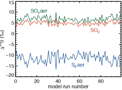
I-d Estimating Δ33S errors in our standard model

As a final check on the data quality of DA08 cross-sections, we performed

two Monte Carlo simulations of our standard atmosphere in which we vary the

SO2 cross section data within their given measurement errors. First, we ran 100

model atmospheres where we randomly selected 3xSO2 cross-section values within the range of measurement errors at each wavelength. This experiment

(not shown) revealed that the predicted DA08 Δ33S magnitudes in our standard

atmosphere are robust to 0.9, 1.5 and 0.6 ‰ in sulfate aerosol, elemental sulfur

aerosol, and SO2 respectively. To form an upper limit on errors, we ran another

100 model atmospheres where we attempted to maximize error at each

wavelength, by randomly selecting either the value, or the value plus the

measurement error or the value minus the measurement error. This experiment,

shown in Figure A4, shows that the predicted DA08 Δ33S magnitudes in our

standard atmosphere are robust to 1.2, 2.1 and 0.9 ‰ in sulfate aerosol,

elemental sulfur aerosol, and SO2, respectively. While the DA08 stated

measurement errors certainly propagate to uncertainty in the predicted

magnitudes, they do not affect our conclusions regarding the sign of Δ33S

produced in the Archean atmosphere. These calculations would not assess if

there were systematic offsets between the various cross-sections (Whitehill and

Ono, 2012). It does, however, confirm that if the DA08 cross-sections are in

Figure A4 – Results from 100 Monte Carlo runs of the standard model where the 3xSO2 were varied maximally (see A1.4 for details).

Appendix II - Additional tests of Halevy et al. (2010)

The predicted Δ33S values in our standard model reflect the radiative

transfer and absorption of solar photons from 180 – 220 nm through the

atmospheric gas column and DA08 cross-sections. Ueno et al. (2009) noted that

any atmospheric gas that absorbs in this wavelength range could modify the Δ33S

signal, by shielding both the quantity and energy of photons available for SO2

photolysis lower in the atmosphere. Furthermore, Ueno et al. (2009) noted that

SO2 photolysis through the DA08 cross-sections with 180 – 200 nm photons

generally yields residual SO2 with a negative Δ33S signal, while SO2 photolysis

0

20

40

60

80

model run number

ï

ï

ï

ï

0

33

S (‰)

)

SO

SO

aer

with 200 – 220 nm photons via DA08 yields residual SO2 with a positive Δ33S

signal. The conventional interpretation of the geologic record is that sulfates are

sourced from this residual SO2 pool, which is converted to sulfate aerosol and

deposited to the surface. Invoking this interpretation, Ueno et al. (2009)

concluded that there must be a strong atmospheric absorber between 200 – 220

nm, so that most of the SO2 photolysis would occur between 180 and 200 nm.

Following up on this interpretation, Halevy et al. (2010) calculated SO2 photolysis

only between 180 and 200 nm, effectively assuming complete opacity of the

atmosphere to photons between 200 and 220 nm. In Figure A5, we find that this

choice does lead to residual SO2 with a negative Δ33S signal with a

correspondingly negative sulfate aerosol. However, we stress that this is not a

self-consistent computation, as photons between 200 and 220 nm should

Figure A5 - A non self-consistent computation of the same atmosphere as shown in Figure 2b, but with Δ33_{S from SO2 photolysis only computed between 180 and 200 nm,} following the assumption of Halevy et al. (2010). This model (along with the fictitious test shown in Fig. A9) is the only model atmosphere in our study which produced negative

Δ33

S sulfate and positive Δ33S sulfur.

Appendix III - Additional model results, including DA08 and the SO2 photoexcitation band

In this section, we present three additional results from our photochemical

models, followed by calculations showing that differential absorption in the SO2

photo-excitation band does not change our primary results.

III-a Additional tests using the Danielache et al. (2008) cross-sections

three figures similar to Figs. 6 and 7, where the independent variables are

biogenic sulfur fluxes (Fig. A6), the CH4/CO2 ratio (Fig. A7), and the CO2 mixing

ratio (Fig. A8).

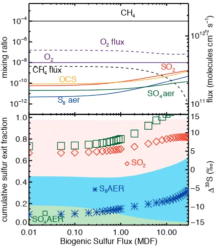
Figure A6 varies the total biogenic sulfur input by scaling the modern

fluxes of CH3SCH3 (dimethyl sulfide), CH3SH (methyl mercaptan), CS2 (carbon

disulfide), and OCS (carbonyl sulfide) from 0.01 to 30 times their modern values,

following the methodology of Domagal-Goldman et al. (2011). In addition to other

species of interest, Figure A6a also shows the ground level OCS concentrations.

In the reducing atmosphere, biogenic sulfur gases tend to be largest near their

source at the ground and fall off with altitude, indicating that the increased loss

pathways arising from enhanced photolysis between 200-300 nm compensates

for the lack of oxidative destruction (Domagal-Goldman et al., 2011). Even at 30

times the modern biogenic sulfur flux, the peak OCS concentration is 1 ppb with

a column depth of ~1016 cm2, far below concentrations needed to shield SO2 photolysis and affect the MIF-S signal (Ueno et al., 2009). Rather, the predicted

Δ33

S changes are due to the increase in total sulfur in the system, which affects

the redox state and exit channels in a manner similar to Fig. 6c/d. The runs in Fig

A6 also contain volcanic sulfur fluxes, so do not show the decrease in reducing

capacity seen in the left most side of Figure 6c/d. As such, the left-most models

of Figure A6 (with volcanic fluxes + 1% of modern biogenic S fluxes) provide the

Figure A6 – Predicted mixing ratios (top panel, left axis, solid lines), fluxes (top panel, right axis, dashed lines), sulfur exit channel fractions (bottom panel, left axis, shaded regions) and Δ33S (bottom panel, left axis, symbols), with colors and symbols as in Figs. 6 and 7. Biogenic sulfur fluxes are varied from 1% of modern to 3000% of modern values.

10

10

10

10

10

mixing ratio

10

10

flux (molecules cm

ï

s

)

CH

O

SO

S

aer

OCS

SO

aer

CH

flux

O

flux

0.01

0.10

1.00

10.00

Biogenic Sulfur Flux (MDF)

0.0

1.0

cumulative sulfur exit fraction

_ï

ï

ï

0

10

33

S (‰)

SO

AER

S

AER

SO

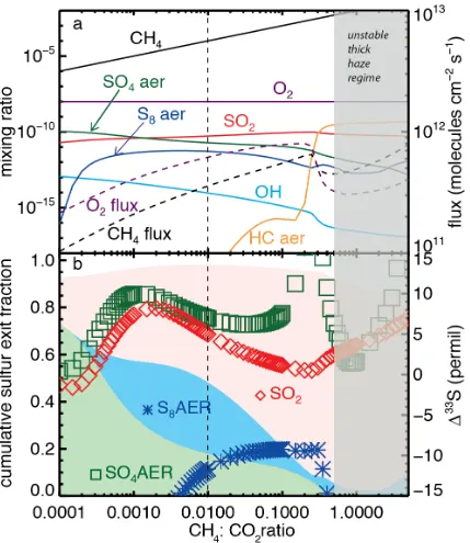
Figure A7a reproduces a Zerkle et al. (2012) model run in which an organic haze

forms when the CH4:CO2 ratio reaches ~0.2, affecting both the chemistry

(Domagal-Goldman et al., 2008; Zerkle et al., 2012) and climate (Haqq-Misra et

al., 2008) of the atmosphere. Figure A7b shows that SO2 becomes the dominant

exit channel and that Δ33S approaches 0‰, consistent with earlier predictions

that an organic haze might explain low Δ33S (Domagal-Goldman et al., 2008).

Large magnitude Δ33S occurs in the SO4 and S8 exit channels in the “thin haze”

regime, although these together comprise less than 20% of the total sulfur flux to

the surface. Interestingly, CH4 concentrations lower than the standard model

(e.g., with 0.005< CH4:CO2 < 0.01) lead to higher magnitude Δ33S in the SO2 and

sulfate channels, with very negative Δ33S in S8. The far left of Fig. A7 represents

increasingly oxic (although still reducing) atmospheres, with Δ33S magnitudes

falling towards 0‰ in the dominant exit channels, as might be expected during

collapsing methane levels prior to the Great Oxidation Event (Kurzweil et al.,

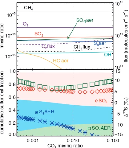
Fig A8 shows that changes in CO2 between modern values and 0.1 bar do not

significantly change Δ33S magnitudes in the SO2 or SO4 exit channels, while the

Δ33

S in S8 drops from -7‰ to -20‰ as the exit channel fraction drops from 50%

to 30%. Negative Δ33S signals of the magnitude predicted at our highest CO2

concentrations are not seen in the geologic record, but these atmospheric MIF

signals are likely diminished en route to sedimentary pyrite and in subsequent

diagenesis (Farquhar et al., 2013; Halevy; Halevy et al., 2010; Lyons, 2009; Ono

et al., 2009). Given the concerns with the data quality of DA08, we conclude that

CO2 is capable of changing atmospheric chemistry enough to perturb Δ33S

signals, even if these specific predictions do not appear to match data from the

Figure A8 – Predicted mixing ratios (top panel, left axis, solid lines), fluxes (top panel, right axis, dashed lines), sulfur exit channel fractions (bottom panel, left axis, shaded regions) and Δ33S (bottom panel, left axis, symbols), with colors and symbols as in Figs. 6 and 7. CO2 mixing ratios are varied from 400 ppm to 10%, with the vertical dashed line indicates the standard model.

10

10

10

mixing ratio

10

10

10

flux (molecules cm

ï

s

)

CH

O

SO

OH

S

aer

HC aer

SO4 aer

CH

flux

O

flux

0.001

0.010

0.100

CO

mixing ratio

0.0

0.2

0.4

0.6

0.8

1.0

cumulative sulfur exit fraction

_ï

ï

ï

0

10

33

S (‰)

SO

AER

S

AER

SO

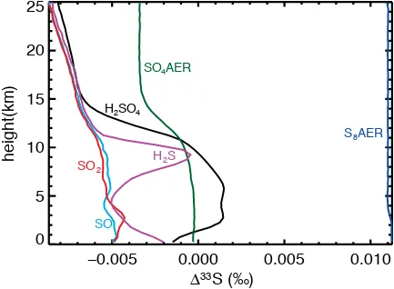
III-b Calculations including the Photoexcitation band (250-320 nm)

The isotopologue cross-sections for the SO2 photoexcitation band have been

recently measured at 8 wavenumber resolution between 250 and 320 nm

(Danielache et al., 2012), including the first published 36SO2 cross-section. In a 1-D atmospheric plume model (with modern levels of oxygen and ozone

rendering the photoylsis band irrelevant), these cross-sections have been shown

to generate time-dependent Δ33S/Δ36S signals on the order of 1‰ when SO2

concentration reach 1 ppm in days to weeks following a large stratospheric

eruption (Hattori et al., 2013). We enhanced our model to include the Danielache

et al. (2012) photoexcitation band cross-sections in addition to the DA08

photolysis band cross-sections, by the expansion of the wavelength grid between

250 and 320 nm to a resolution of 0.05 nm. Re-running the standard model with

both the photolysis and photoexcitation bands active, we predict only minor

changes in our predicted Δ33S values (Table 1). The magnitudes of the

quantitatively significant exit channels decrease (towards zero), implying that the

net effect of the differential absorption due to amplitude variations within the

photoexcitation band in a reducing atmosphere is to drive sulfates negative and

sulfides positive. This behavior is confirmed by a non-self consistent model

calculation in which we only integrate the 3xSO2 cross-sections from 250-320 nm.

This model, shown in Figure A9, produces low magnitude positive Δ33S in the S8

(2013), except for the low magnitudes. The maximum predicted SO2 mixing ratio

is ~0.5 ppb in the lower stratosphere (Fig 2a), so we assume our lower Δ33S

magnitudes are due to the 4 orders of magnitude less SO2 in our atmospheric

column. Very recently, larger magnitude Δ33S signals were produced in laboratory

experiments probing the photoexcitation band, and attributed to enhanced

lifetimes for excited species, independent of their excitation wavelength (Whitehill

et al., 2013). This mechanism, along with that of SO2 self-shielding in optically

thick SO2 plumes (Lyons, 2009; Ono et al., 2013) is beyond the scope of our

current calculations but may be important for future efforts.

Figure A9 – A non self-consistent computation of Archean photochemistry including only the isotopic effect of the 250-320 nm photoexcitation band.

ï

height(km)

33

_{S (‰)}

)

SO

AER

S

AER

H

S

H

SO

SO

References:

Claire, M.W., Catling, D.C., Zahnle, K.J., 2006. Biogeochemical Modeling of the Rise in Atmospheric Oxygen. Geobio 4, 239-269.

Danielache, S.O., Hattori, S., Johnson, M.S., Ueno, Y., Nanbu, S., Yoshida, N., 2012. Photoabsorption cross-section measurements of S-32, S-33, S-34, and S-36 sulfur dioxide for the B1-X1A1 absorption band. J. Geophys. Res. - Atm 117.

Domagal-Goldman, S., Johnston, D., Farquhar, J., Kasting, J.F., 2008. Organic Haze, Glaciations, and Multiple Sulfur Isotopes in the Mid-Archean Era. Earth Planet. Sci. Lett. 269, 29-40.

Domagal-Goldman, S., Meadows, V., S., Claire, M.W., Kasting, J.F., 2011. Using Biogenic Sulfur Gases as Remotely Detectable Biosignatures on Anoxic Planets. Astbio 11, 1-23.

Farquhar, J., Cliff, J., Zerkle, A.L., Kamyshny, A., Poulton, S.W., Claire, M., Adams, D., Harms, B., 2013. Pathways for Neoarchean pyrite formation constrained by mass-independent sulfur isotopes. Proc. Natl. Acad. Sci. U. S. A.

Farquhar, J., Johnston, D.T., Wing, B.A., 2007. Implications of conservation of mass effects on mass-dependent isotope fractionations: Influence of network structure on sulfur isotope phase space of dissimilatory sulfate reduction. Geochim. Cosmochim. Acta 71, 5862-5875.

Goldblatt, C., Lenton, T.M., Watson, A.J., 2006. Bistability of atmospheric oxygen and the Great Oxidation. Nature 443, 683-686.

Halevy, I., 2013. Production, preservation, and biological processing of

mass-independent sulfur isotope fractionation in the Archean surface environment. Proc. Natl. Acad. Sci. U. S. A.

Halevy, I., Johnston, D.T., Schrag, D.P., 2010. Explaining the Structure of the Archean Mass-Independent Sulfur Isotope Record. Science 329, 204-207.

Haqq-Misra, J.D., Domagal-Goldman, S.D., Kasting, P.J., Kasting, J.F., 2008. A Revised, Hazy Methane Greenhouse for the Archean Earth. Astbio 8, 1-11.

Hattori, S., Schmidt, J.A., Johnson, M.S., Danielache, S.O., Yamada, A., Ueno, Y., Yoshida, N., 2013. SO2 photoexcitation mechanism links mass-independent sulfur isotopic fractionation in cryospheric sulfate to climate impacting volcanism. Proc. Natl. Acad. Sci. U. S. A.

Johnston, D.T., 2011. Multiple sulfur isotopes and the evolution of Earth's surface sulfur cycle. Earth-Sci Rev 106, 161-183.

Kurzweil, F., Claire, M., Thomazo, C., Peters, M., Hannington, M., Strauss, H., 2013. Atmospheric sulfur rearrangement 2.7 billion years ago: Evidence for oxygenic photosynthesis. Earth Planet. Sci. Lett. 366, 17-26.

Lyons, J.R., 2009. Atmospherically-derived mass-independent sulfur isotope signatures, and incorporation into sediments. Chem. Geol. 267, 164-174.

Ono, S., Whitehill, A.R., Lyons, J.R., 2013. Contribution of isotopologue self-shielding to sulfur mass-independent fractionation during sulfur dioxide photolysis. J. Geophys. Res. - Atm 118, 2444-2454.

Ono, S.H., Beukes, N.J., Rumble, D., 2009. Origin of two distinct multiple-sulfur isotope compositions of pyrite in the 2.5 Ga Klein Naute Formation, Griqualand West Basin, South Africa. Precambrian Res. 169, 48-57.

Pavlov, A.A., Kasting, J.F., 2002. Mass-independent fractionation of sulfur isotopes in Archean sediments: strong evidence for an anoxic Archean atmosphere. Astbio 2, 27-41.

Ueno, Y., Johnson, M.S., Danielache, S.O., Eskebjerg, C., Pandey, A., Yoshida, N., 2009. Geological sulfur isotopes indicate elevated OCS in the Archean atmosphere, solving faint young sun paradox. Proc. Natl. Acad. Sci. U. S. A. 106, 14784-14789. Whitehill, A.R., Ono, S., 2012. Excitation band dependence of sulfur isotope mass-independent fractionation during photochemistry of sulfur dioxide using broadband light sources. Geochim. Cosmochim. Acta 94, 238-253.

Whitehill, A.R., Xie, C., Hu, X., Xie, D., Guo, H., Ono, S., 2013. Vibronic origin of sulfur mass-independent isotope effect in photoexcitation of SO2 and the implications to the early earths atmosphere. Proc. Natl. Acad. Sci. U. S. A.

Zahnle, K.J., Claire, M.W., Catling, D.C., 2006. The loss of mass-independent fractionation in sulfur due to a Paleoproterozoic collapse of atmospheric methane. Geobio 4, 271-283.