Identifying prognostic structural features in tissue sections of colon cancer patients using point pattern analysis

DOI: xxx/xxxx

ARTICLE TYPE

Identifying prognostic structural features in tissue sections of

colon cancer patients using point pattern analysis

†

Charlotte M. Jones-Todd*

_{| Peter Caie**}

_{| Janine B. Illian}

_{| Ben C. Stevenson}

_{| Anne}

Savage

_{| David J. Harrison}

_{| James L. Bown}

1_{National Institute of Water and}

Atmospheric Research, New Zealand and Centre for Research into Ecological&

Environmental Modelling, School of Mathematics and Statistics, University of St Andrews, UK

2_{School of Medicine, University of St}

Andrews, UK

3_{Centre for Research into Ecological&}

Environmental Modelling, School of Mathematics and Statistics, University of St Andrews, UK

4_{Department of Statistics, University of}

Auckland, New Zealand

5_{School of Science, Engineering and}

Technology, Abertay University, UK

6_{School of Arts, Media and Computer}

Games, Abertay University, UK

Correspondence

*Charlotte M. Jones-Todd, NIWA, Gate 10 Silverdale Road, Hillcrest, Hamilton, NZ Email: [email protected] **Peter Caie, School of Medicine, University of St Andrews, KY16 9TF, UK Email: [email protected]

Abstract

Diagnosis and prognosis of cancer is informed by the architecture inherent in

can-cer patient tissue sections. This architecture is typically identified by pathologists,

yet advances in computational image analysis facilitate quantitative assessment of

this structure. In this article we develop a spatial point process approach in order

to describe patterns in cell distribution within tissue samples taken from colorectal

cancer (CRC) patients. In particular, our approach is centered on the Palm intensity

function. This leads to taking an approximate-likelihood technique in fitting point

processes models. We consider two Neyman-Scott point processes and a void

pro-cess, fitting these point process models to the CRC patient data. We find that the

parameter estimates of these models may be used to quantify the spatial arrangement

of cells. Importantly, we observe characteristic differences in the spatial arrangement

of cells between patients who died from CRC and those alive at follow-up.

KEYWORDS:

Colorectal cancer; Palm intensity function; Spatial point patterns

1

INTRODUCTION

A fundamental aspect of cancer patient diagnosis and prognosis concerns the assessment by pathologists of histopathologi-cal architectural and morphologihistopathologi-cal properties within patient tissue sections. These sections typihistopathologi-cally comprise both cancerous (tumour), and non cancerous (e.g., stroma) tissue structures, with regions of each intermixed in space.1_{Pathologists categorise} tumours into stages that are associated with the progression of the cancer and patient outcome. Cancer staging is good at pre-dicting population survival statistics but not as accurate at prepre-dicting an individual patient’s prognosis.2 _{This is due, in part,} to complex tumour heterogeneity and a lack of histopathological features within the tissue which can be reliably identified and reproducibly quantified by eye. The pattern of invasive growth in colorectal cancer (CRC) has been previously linked to the level of aggressiveness of the disease and patient prognosis.3,4,5 _{The phenomenon of tumour budding, where small distinct}

†_{Point pattern analysis of colon cancer tissue sections.}

islands of tumour cells are widely dispersed within the stroma at the invasive front of CRC, has been shown to be prognostically significant.6,7

Advances in computational image analysis provide an opportunity for quantitative and objective assessment of tissue mor-phology. In previous work,8_{the focus of investigation was on the morphological pattern of the tumour and no consideration was} given to the spatial arrangement of cells. In particular, image analysis methodology was found to standardise the quantification of histopathological features (e.g., tumour budding, lymphatic vessel density, and lymphatic vessel invasion) within the invasive front of the tissue section.

The importance of the tissue architecture for tumour grading is recognised where in previous work the spatial patterning of cells was characterised and used as an indicator of patient outcome.1 _{This was achieved through considering the locations} of cells as a point pattern—a realisation of a spatial point process. In particular, this work compared a first-order statistic, the estimated point process intensity, and two second-order statistics, the pair correlation function and Ripley’s K-function, between two patient groups: patients whose cancer had and had not metastasised, a major indicator of patient survival. Results, however, showed no differences between patient groups with respect to first- or second-order spatial statistics and the authors recognised that standard statistical spatial point process methods do not adequately capture the spatial architecture of cancerous tissue.

In reality, cancerous tissue is a result of many complex processes resulting in obscure spatial structures capturing the inter-mixing of cancerous and non-cancerous cells. The morphology of the tissues reflects some of this complexity and as such we propose that these particular methods were perhaps too simplistic and relied on assumptions (e.g., homogeneity) that do not hold and therefore failed to capture the spatial structure of the tissue sections. Characterising the spatial structure of cells is nontriv-ial and requires the use of more complex, nonstandard, spatnontriv-ial point process methodology. In the following sections we develop spatial point process methodology that characterises the spatial arrangement of tissue using the interpoint distances between cells to inform consideration of the spatial morphology of CRC tissue.

1.1

Characterising the structure of parent-daughter point processes

In order to present the spatial point process methodology and, in particular, the point process models developed herein we consider two types of points,parentanddaughterpoints. Note that these donotrefer to the distinction between tumour and stroma cells; rather parent and daughter points areabstractconstructs. A classic example of a parent-daughter process is the Neyman-Scott point process (NSPP), which is acluster process. Here, the parent points, themselves generated by a homogeneous Poisson process, randomly generate daughters centered at their unobserved locations.9_{We propose an additional process that} relies on unobserved parents, which we call avoid process. In a void process, observed points are a realisation of a homogeneous point process, but those within some fixed distance of an unobserved parent are deleted. To define a void process, we consider two homogeneous Poisson processes X and P. The realisation of P is a pattern that forms the centroid locations,𝑝∈P, of circular voids of radius𝑅 >0. Through superimposing P on X then any𝑥∈X that fall with the voids are deleted. The resulting pattern is the observed void point pattern, a realisation of the void process (see Appendix A.1 for further details).

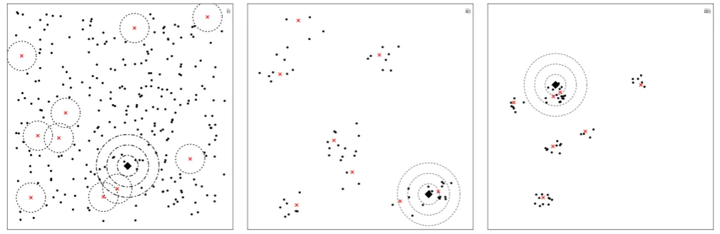
Figure 1 plot𝑖)shows a realisation of a void process and plots𝑖𝑖)and𝑖𝑖𝑖)show two realisations of NSPPs—a Thomas and a Matérn process, respectively. The difference between a Thomas and a Matérn process is the dispersion of daughter points around their parents. In the case of a Thomas process the spatial locations of daughters around their parents follows a bivariate normal distribution and in the case of a Matérn process the daughters are uniformally distributed in a circle around their parents.

In all the processes discussed above the parent points are a realisation of a homogeneous Poisson point process with intensity 𝐷. Each process is characterised by two further parameters that relate to the daughter points. In the case of the void process we define these as𝜆, the intensity of daughters prior to deletion, and𝑅, the radius of the voids. Hence, the parameter vector of a void process is given by𝜽= (𝐷, 𝑅, 𝜆).

In the case of the Neyman-Scott point process we define the parameter vector as𝜽= (𝐷, 𝜙, 𝛾). The number of daughters sired by a parent is assumed to be Poisson with expectation𝜙. In addition, conditional on their parent’s locations, the daughters are scattered in space according to some distribution with parameter𝛾. In the case of a Thomas process the variance-covariance matrix for the bivariate Gaussian distribution of daughters around their parents is given by𝛾2𝐈₂In the case of a Matérn process, 𝛾 is the radius of the circle, centered at the location of a parent point, within which daughters are uniformally scattered.

parent and so other points are likely to be nearby as they are safe from deletion. As𝑟increases, the fraction of the circle𝑏(𝑥, 𝑟)

that intersects with a void is likely to increase, thus decreasing point density within it. For further details see Appendix A. In the following sections we describe parameter estimation for void, Thomas, ans Matérn processes. Thomas processes have previously been fitted via maximisation of the Palm likelihood functions10,11and we extend this approach to void and Matérn processes. In Section 3 we present the results of the application of our approach to a CRC patient data set.2,8

FIGURE 1i) A simulated void processes in the unit square. Daughter points are generated by a homogeneous Poisson process and are deleted if they fall within circular voids, of radius𝑅 = 0.075, centered at parent points (red crosses, unobserved in practice). The remaining daughters (black dots) have intensity given by𝜆 = 300. The number of parents simulated are IID following a Poisson distribution with expectation 𝐷 = 10. The dotted circles indicate the simulated voids. Considering an arbitrarily chosen daughter (encircled diamond) then there are more likely to be nearby daughters as that chosen daughter is not within a void. The dashed circles show how the intensity of observed daughters changes for different distances𝑟, radius of the circle, away from an arbitrary point (i.e., the density of daughters is higher nearer the chosen point, but further away a void is more likely to be encountered and therefore the density decays). Plots ii), Thomas, and iii), Matérn, show two simulated Neyman-Scott point processes in the unit square with unobserved parent points (red crosses) siring the observed daughters (black dots). In each case parents are generated by a homogeneous Poisson process with intensity𝐷= 7. The number of daughters sired by each parent are IID Poisson with expectation𝜙= 8. In each case𝛾 = 0.05. In ii) daughters are dispersed around their parents due to a bivariate normal distribution,𝐍₂(𝟎, 𝛾2_𝐈

2); in iii) the daughters are uniformally distributed around their parents in a circle

with radius𝛾. Here, again, the dashed circles show how the intensity of observed daughters changes for different distances𝑟, radius of the circle, away from an arbitrary point (encircled diamond); the density of daughters is higher nearer the chosen point, but further away points in the sibling cluster are less likely to be encountered and therefore the density decays.

2

A PALM LIKELIHOOD APPROACH FOR PARAMETER ESTIMATION

The following subsections derive the Palm intensity for two-dimensional void processes (Section 2.1), detail the derivation of the Palm intensity for the Thomas process,11_{and generalise this to the Matérn Palm intensity (Section 2.2). The full derivation} of these Palm intensities in general𝑑dimensions is given in Appendix A.

2.1

Void point process Palm intensity

The Palm intensity of a void process may be formulated as the product of the global point density of the pattern prior to deletion, 𝜆, and𝑝𝑠(𝑟), the probability that a potential point at distance𝑟is within a distance𝑅of an unobserved parent and is therefore safe from deletion.

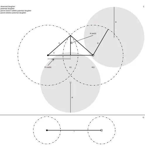
This probability is related to the geometry of the intersection between two circles of common radius𝑅centered at an observed daughter and a potential daughter point. This is illustrated in more detail in Figure A.1 in the Appendix. The intersection,𝐼(𝑟), between two circles centered at an observed daughter and a potential daughter respectively is the only region we know a parent cannot exist within𝑅of the potential daughter. The remaining area,𝐴(𝑟), of the circle centered at the potential point is the only region which may contain a parent whose void would delete that potential daughter. The potential daughter is safe from deletion if there are no parents in the region𝐴(𝑟). Parents are generated by a homogeneous Poisson point process with intensity 𝐷therefore this occurs with probability

𝑝_𝑠(𝑟) =exp(−𝐷 𝐴(𝑟)),

In 2 dimensions𝐴(𝑟) =𝜋𝑅2_{−𝐼(𝑟). This area can be determined through the use of elementary geometry, detailed in Appendix}

A.1.14

The area of intersection,𝐼(𝑟), between two circles with a common radius R is given by,

𝐼(𝑟) =𝜋 𝑅2I (

1 −( 𝑟 2𝑅

)2

;3 2,

1 2

)

. (1)

Here I(𝑧;𝑎, 𝑏) = 𝐵_𝐵(𝑧;𝑎,𝑏)

(𝑎,𝑏) is the regularised Beta function. The Palm intensity function is then derived as,

𝜆(𝑟;𝜽) =𝜆𝑝_𝑠(𝑟),

=𝜆exp (

−𝐷 𝜋 𝑅2 [

1 −I (

1 −( 𝑟 2𝑅

)2

;3 2,

1 2

)]) ,

=𝜆exp(−𝐷 𝜋 𝑅2 [1 −F_𝑔(𝑟)(3

2, 1 2

)]) ,

(2)

where𝑔(𝑟) = 1 −( 𝑟

2𝑅

)2

, and F_𝑔(𝑟)(⋅,⋅)is the CDF of the Beta distribution. Note when𝑟 = 0⇒𝑔(𝑟) = 1⇒F₁(⋅,⋅) = 1⇒

𝜆(0;𝜃) = 𝜆, the intensity of daughters prior to deletion. In addition, when𝑟 = 2𝑅⇒𝑔(𝑟) = 0⇒F₀(⋅,⋅) = 0⇒𝜆(0;𝜃) =

𝜆exp(−𝐷 𝜋 𝑅2_{), due to the properties of the CDF. For the full derivation of the Palm intensity (2) see Appendix A.1.}

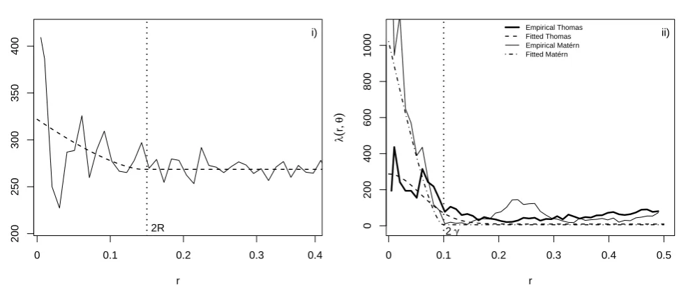
Figure 2, plot i), shows both the empirical Palm intensity function (solid line),15 _{and the fitted Palm intensity (dashed line)} for the simulated void process shown in Figure 1. The Palm intensity is a piece-wise continuous function with two sub-domains

(0,2𝑅],[2𝑅,∞). The horizontal asymptote to which the Palm intensity decays is the baseline intensity.

2.2

Neyman-Scott point process Palm intensity

The Palm intensity function of a Neyman-Scott point process (in 2 dimensions) is given by10

𝜆(𝑟;𝜽) =𝐷 𝜙+ 𝜙 𝑓𝑦(𝑟;𝛾)

2𝜋 𝑟 , (3)

where the parameter𝐷is the intensity of parents. Letting𝑌 denote the distance between two randomly selected sisters (i.e., daughters sired by the same parent) then𝑓𝑦(𝑟;𝛾)is the PDF of𝑌 and is characterised by the parameter𝛾pertaining to the form of distribution of daughters around their parents.

The Palm intensity of a modified Thomas process is a special case of Equation (3) where (i) parent locations are realisations of a homogeneous Poisson process, (ii) the numbers of daughters sired by each parent are Poisson IID, and (iii) daughters are dispersed due to a bivariate normal distribution .11_{The analytic Palm intensity for a modified Thomas process is given by}

𝜆(𝑟;𝜽) =𝐷 𝜙+ 𝜙 4𝜋𝛾2exp

(

−𝑟2

4𝛾2

)

0 0.1 0.2 0.3 0.4

200

250

300

350

400

i)

r

λ

(

r

, θ

)

2R

0 0.1 0.2 0.3 0.4 0.5

0

200

400

600

800

1000

r

λ

(

r

, θ

)

ii) Empirical Thomas

Fitted Thomas Empirical Matérn Fitted Matérn

2 γ

FIGURE 2Both the empirical15 (solid lines) and fitted (dashed lines) Palm intensities for the simulated patterns shown in Figure 1. The fitted intensities were estimated using the methods discussed herein. The Palm intensity for the void process, parametrised as𝜽 = (𝐷, 𝑅, 𝜆) = (10,0.075,300), is shown in plot i). This is a piece-wise continuous function with two sub-domains (0,2𝑅],[2𝑅,∞). The Palm intensities for both the simulated Neyman-Scott point processes, parametrised as𝜽 = (𝐷, 𝜙, 𝛾) = (10,8,0,05), are shown in plot ii). Here, the Matérn cluster process decays at a much steeper rate due again to it being a piece-wise continuous function with two sub-domains(0,2𝛾],[2𝛾,∞). The vertical dotted lines in each plot indicate where𝑟= 2𝑅for the void process and𝑟= 2𝛾for the Matérn process.

Thus,𝜆(𝑟;𝜽)is the sum of the intensity of non-sister points,𝐷 𝜙, and a Gaussian function describing the intensity due to sister points. For a Thomas process, the PDF of𝑌 is the distance between two normally distributed sisters. For example, in Equation 4,

𝑓𝑦(𝑟;𝛾) =

𝑟exp(−𝑟2_∕(4𝛾2₎₎

2𝛾2 , (5)

where𝛾, is the parameter describing the Gaussian dispersion of daughters around their parents.

For the Matérn process,𝑓_𝑦(𝑟;𝛾)is now the PDF of the distance between two sisters generated from a uniform distribution within a circle of radius𝛾. This PDF16_{is given by}

𝑓_𝑦(𝑟;𝛾) = 4

𝐵(3

2, 1 2)

𝑟 𝛾3 ×

[

2𝐹1

(₁

2,− 1 2,

3 2,1

) 𝛾−₂𝐹₁

(

1 2,−

1 2,

3 2,

𝑟2

4𝛾2

) 𝑟

2

] ,

= 4𝑟∫𝑟𝛾

2

(𝛾2_−𝑥2₎12𝑑𝑥

𝐵(3

2, 1 2)𝛾

4 .

(6)

Here𝐵(⋅,⋅)denotes the beta function, and₂𝐹₁(⋅,⋅,⋅,⋅)is the hyper-geometric function. For derivation of this see Appendix A.2.16 The empirical and fitted Palm intensities for the simulated Neyman-Scott point processes in Figure 1 are depicted in Figure 2. Both simulated processes in Figure 1, plots ii) and iii), were generated with parameter values𝜽= (𝐷, 𝜙, 𝛾) = (7,8,0.05). The Palm intensities in each case decay to the same asymptote, the baseline intensity𝐷𝜙.

2.3

The Palm likelihood for point process models

structure of the cell nuclei, does not simply terminate at the image’s edge. This is an issue that arises in the modelling of any spatial point pattern and there are a number of approaches to address it.12 _{Our approach calculates distances between points} subject to periodic boundary conditions and as such we are required to set a truncation distance,𝑡.11,10_{This is set to a distance} that is larger than any plausible distance between two sisters, or between parents in the void process case.

Taking an approximate-likelihood approach, the estimator for the parameter vector𝜽is given by

̂

𝜽=arg max_𝜽𝐿(𝜽;𝐫),

where𝐿(𝜽;𝐫)is the Palm likelihood. Through the numerical maximisation of log(𝐿(𝜽;𝐫)), with respect to𝜽,𝜽̂ is evaluated. The Palm likelihood,𝐿(𝜽;𝐫), is given by

𝐿(𝜽;𝐫) =

⎛ ⎜ ⎜ ⎝

∏

{𝑖,𝑗∶||𝑥𝑖−𝑥𝑗||<𝑡,𝑖≠𝑗}

𝑛 𝜆(𝑟;𝜽)

⎞ ⎟ ⎟ ⎠ exp ⎛ ⎜ ⎜ ⎝ −𝑛 𝑡 ∫ 0

𝜆(𝑟;𝜽) 2𝜋 𝑟d𝑟 ⎞ ⎟ ⎟ ⎠

. (7)

Here the product is that taken over all𝑛distinct observed pairs of points,𝑥𝑖, 𝑥𝑗 (𝑖≠ 𝑗), where the distance between them, ||𝑥_𝑖−𝑥𝑗||, is less than the truncation distance𝑡.10,11_{The integral term may be simplified for each process discussed herein; this} results in an objective function that is very computationally efficient to compute. Simplifications of this integral are given for each process below.

• Void process. The integral, given in the likelihood (7), for the void process is derived as,

𝑡

∫

0

𝜆(𝑟;𝜽) 2𝜋 𝑟d𝑟=𝜆2𝜋exp(−𝐷 𝜋 𝑟2) 𝑡

∫

0

exp(𝐷 𝜋 𝑟2F_𝑔(𝑟)(1,1

2

)) 𝑟d𝑟.

This is intractable as it contains the CDF of a Beta distribution, F_𝑔(𝑟)(⋅,⋅), where𝑔(𝑟) = 1 −( 𝑟

2𝑅

)2

. In our estimation procedure F_𝑔(𝑟)(⋅,⋅)is computed numerically.

• Neyman-Scott point processes. The integral given in likelihood (7) simplifies to,

𝑡

∫

0

𝜆(𝑟;𝜽) 2𝜋 𝑟d𝑟=𝐷 𝜙+𝜙 𝐹_𝑦(𝑡;𝛾),

where𝐹𝑦(𝑡;𝛾)is the CDF of the distance between two randomly selected sisters, which can be derived by taking the first derivative of𝑓_𝑦(𝑡;𝛾)(Section 2.2) with respect to𝑡. Below we give𝐹_𝑦(𝑡;𝛾)for each case of the Neyman-Scott point process.

– Matérn cluster process

𝐹_𝑦(𝑡;𝛾) = 𝑡2

𝛾2 ⎛ ⎜ ⎜ ⎜ ⎝ 1 −

𝐵_𝛼(1

2, 3 2

)

𝐵(1

2, 3 2 ) ⎞ ⎟ ⎟ ⎟ ⎠ + 4

𝐵_𝛼(3

2, 3 2

)

𝐵(1

2, 3 2

),

where𝐵_𝛼(⋅,⋅)and𝐵(⋅,⋅)are the incomplete beta function and the beta function respectively. That is,𝐵(𝛼;𝑎, 𝑏) =

∫₀𝛼𝑢(𝑎−1)_{(1 −𝑢)}(𝑏−1)_{𝑑𝑢and for𝛼= 1𝐵(𝛼;𝑎, 𝑏) =𝐵(𝑎, 𝑏). The derivation of these equations is detailed in Appendix}

A.2.

– Thomas cluster process

Again letting𝑦 be the Euclidean distance between two randomly selected daughters (the locations of whom are independent given the the parent locations) then𝑦 =𝛾_𝜒√2, which is strictly monotonic. Here for two-dimensions

𝜒 =√𝜒2_{∼chi(2) where𝜒}2_{∼chi-squared(2) and the CDF is given by,}10

𝐹_𝑦(𝑡;𝛾) =𝑃 (

1, 𝑞

2

4𝛾2

)

3

SPATIAL POINT PROCESS MODELS FOR CRC DATA

The data analysed in this article refer to forty two patients drawn from a wider data set of a pan-Scotland cohort of patients, diagnosed with CRC.8_{In the subset of data we analyse twenty three patients that survived CRC and nineteen that had died at} follow up due to CRC. Follow up was a maximum of fourteen and a quarter years post surgery, see Appendix A.3 Table A3 for further details. In addition, the severity of the cancerous tissue was graded by a pathologist as either Dukes A (least severe), Dukes B, or Dukes C (most severe). All patients graded Dukes A were alive at follow up and those graded Dukes C were all dead at follow up; the patients graded Dukes B consisted of a mixture (∼ 50%)of patients who died from CRC and were alive at follow up.

Each patient had up to fifteen fields of view captured, using a x20 objective, from the invasive front of the tissue section. Images were captured using a DAKO link 48 platform, which automates manual immunofluorescence staining. Set exposure times and imaging profiles were utilised to capture each fluorophore during image capture. These images were then processed by an automated imaging algorithm implemented in Definiens Developer XDTMthat segmented the cancer from stroma and segmented each individual nucleus across an image. A panCytokeratin antibody, whose antigen is expressed in CRC cells, was used to visualise each cancer cell. This fluorescence visualisation was input to train a machine learning algorithm within the Definiens software to automatically detect all cancer cells and segment them from the stromal cells. Post tumour to stroma segmentation the DAPI fluorescence was utilised to segment each nucleus in the image. Definiens’ hierarchical image analysis approach allowed the classification of each nucleus to be only assigned to either a cancer cell or a stromal cell. Finally the x-, y-spatial coordinates from the centre of each classified nucleus was exported from Definiens and was used as input for the point process models.

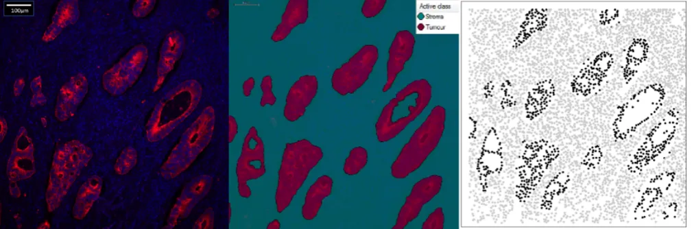
Plot iii) in Figure 3 illustrates, for one patient, the observed point pattern of cells within a tissue section obtained from the digital image shown in plot i). The procedure for going from plot i) to plot iii) in Figure 3 for each slide required the use of an automatic imaging algorithm, detailed above.2In summary, distinct regions in the digitised tissue section were first divided into four types through machine learning: (i) tumour, (ii) stroma, (iii) necrosis/lumen and (iv) no tissue. Plot iii) of Figure 3 shows the point pattern formed by the tumour and stroma cell nuclei, black and grey, respectively, of the same tissue section. From this we see that the morphological patterns within tissue sections, at the very least, (i) are non-homogeneous, and (ii) exhibit complex spatial morphology.

FIGURE 3Illustration of one image of a patient’s slide which enables the pinpointing of nuclei. Plot i) is a composite immunoflu-orescence digital image (red fluimmunoflu-orescence highlights tumour cells and blue fluimmunoflu-orescence highlights all nuclei in the image). Plot ii) is an image analysis mask overlay from automatic machine learnt segmentation of the digital image: tumour (purple), and stroma (turquoise). Plot iii) is the point pattern formed by the nuclei of the tumour (black) and stroma (grey) cells shown in the previous two images.

intermixing of tumour and stroma, or necrosis. We therefore take a nonstandard spatial point process approach using the Palm intensity function to characterise the structure of the tissue sections. We consider maximum Palm likelihood estimation for three point processes: a void process, a Thomas process, and a Matérn process. The parameters of these processes are then considered to represent characteristics of the tissue structure, and are estimated via maximisation of the Palm likelihood, see Section 2.3.

We implemented the methods described in Section 2 in the R packagepalm,17 _{which is available on CRAN. Appendix C} gives and example of its use in the context of the CRC data. In addition, online supplementary material illustrating the fitting of the model discussed in this article may be found at https://github.com/cmjt/examples/blob/master/CRC_point_process.md.

3.1

Results

Each of the point processes discussed give rise to different structures in point pattern data. The parameters in each process therefore reflect different aspects of the morphology of the tissue sections. Having fitted the models discussed above to the CRC data in this section we investigate whether the estimated point process parameters aid in discriminating between patient mortality outcomes (i.e., dead from disease or alive at follow up). We also determine whether patient staging (i.e., Dukes A, Dukes B and Dukes C) falls in line with the structure inferred by the parameter estimates.

We estimate parameters at the patient level for each tumour and stroma pattern by taking the product of the likelihood in Equation (7) over the multiple patterns (images) for each patient. These paramaters are summarised for each i) Dukes staging and ii) patient outcome group by the mean and associated 95% confidence interval, which are calculated using one thousand bootstrap resamples.

To identify parameters that might enable us to discriminate between patient mortality at follow up we use a permutation test with 9999 resamples. Our permutation test statistic is the magnitude of the difference between means, of the chosen parameter, for each patient outcome (i.e., “Alive” or “Died”). Formally this relates to a null hypothesis given by𝐻₀∶|𝜇𝐷𝑖𝑒𝑑−𝜇𝐴𝑙𝑖𝑣𝑒|= 0 and a two-sided alternative hypothesis of𝐻₁ ∶ |𝜇_{𝐷𝑖𝑒𝑑} −𝜇𝐴𝑙𝑖𝑣𝑒| ≠ 0. This permutation test is thus a non-parametric version of a t-test. We correct for multiple tests using two correction methods:⋆Bonferroni correction and⋄a false discovery rate correction.18_{The Bonferroni method is notoriously conservative controlling the family-wise error rate (i.e., the overall chance} of rejecting the null hypothesis when it is true). The false discovery rate method we use holds for independent p-values with non-negative association controlling the expected proportion of false discoveries amongst the rejected hypotheses.

In addition, we use survival analysis to take into account patient follow up time, fitting Cox proportional hazard models19 using each estimated parameter as a predictor. Table C1 in Appendix A3 gives the full results of these models.

Finally, we use our fitted models to explore the suitability of the NSPP and void point processes for capturing the underlying complexities of the cell distributions. We do this by using the empty space function, a functional summary characteristic of point patterns, to compare the fitted models to both the theoretical Poisson process and data simulated with the fitted parameter values.

3.1.1

Estimated parameters of the void process

A void, in the context of spatial point patterns, is a region that contains no point where, given the general structure of the data, points may be expected. This section assumes that each of the separate point patterns formed by tumour and stroma nuclei are realisations of void processes. Therefore, the void process describing the tumour cell point pattern reflects the patterning of stroma cells and vice versa; note the void processes also reflect the less frequently occurring regions of necrosis/lumen and no tissue.

Table 1 summarises the bootstrap resamples of the fitted void process parameters; parent density,𝐷̂, child density,𝜆̂, and void radii,𝑅̂. Table 1 show the averages and the associated 95% confidence interval for each Dukes stage and patient mortality group at follow up. The quoted p-values refer the permutation test discussed above.

The permutation test (using the false discovery rate correction) indicates that in respect of discriminating between patient mortality outcomes find that

(i) There is strong evidence (p-value 0.007) to suggest that stroma daughter density,𝜆̂, in patients that died was lower than in those that were alive at follow up. In addition, there is weak evidence (p-value 0.086) to suggest that stroma parent density,

̂

𝐷, in patients that died was lower than in those that were alive at follow up. This is also indicated by the results of the Cox proportional hazard models where the hazard ratios were estimated respectively as HR= 0.477, CI(0.277,0.820), and HR

(ii) There is weak evidence (p-value 0.086) to suggest that tumour daughter density,𝜆̂, in patients that died was higher than in those that were alive at follow up. Using Cox proportional hazard the results also indicate that patients with higher (scaled) daughter density are more likely to die, HR= 1.352, CI(1.086,1.685).

These results also align with the patient’s Dukes grading. This would be as we would expect due to all patients graded C dying from CRC and all patients graded A being alive at follow up. For example, stroma nuclei patterns of patients graded Dukes C had on average a lower parent and daughter density than those graded Dukes A. The difference is less clear when considering patients graded Dukes B; this we might expect as Grade B patients were a mixture (∼ 50%) of patients who died from CRC and those still alive at follow up.

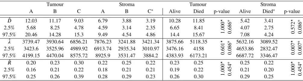
TABLE 1Summaries of the bootstrap resamples for parameters of the void process. These are summarised by the mean value and

95%confidence intervals for both tumour and stroma patterns at each Dukes grade, A, B, and C, and patient mortality at follow up, Alive or Died. The p-values relate to a permutation test as follows:𝐻₀ ∶|𝜇_{𝐷𝑖𝑒𝑑}−𝜇𝐴𝑙𝑖𝑣𝑒|= 0vs𝐻₁∶|𝜇_{𝐷𝑖𝑒𝑑}−𝜇𝐴𝑙𝑖𝑣𝑒|≠0. To adjust for multiple comparisons we use both the Bonferroni correction method and a false discovery rate correction. These are denoted by the superscripts⋆and⋄respectively.

Tumour Stroma Tumour Stroma

A B C A B C∗ _{Alive Died p-value Alive Died}∗ _p-value

̂

𝐷 12.03 11.17 9.03 6.79 3.88 3.19 10.28 11.85

1.000

⋆

0.686

⋄ 5.42 3.41

0.572

⋆

0.086

⋄

2.5% 5.68 8.25 4.78 4.59 3.14 2.35 6.65 8.41 4.07 2.75

97.5% 20.46 14.28 15.3 9.49 4.54 4.86 14.4 15.67 7.08 4.24

̂

𝜆 3739.47 3930.64 6856.21 7876.23 3241.88 3421.34 3875.66 5118.35

0.601

⋆

0.086

⋄ 5632.16 3089.52

0.007

⋆

0.007

⋄

2.5% 3423.6 3525.96 4989.92 6913.74 2935.34 3010.97 3476.16 4158 4653.86 2832.47 97.5% 4199.15 4470.04 8575.72 8925.9 3531.47 3884.2 4383.93 6173.21 6687.72 3346.47

̂

𝑅 0.20 0.23 0.30 0.22 0.25 0.22 0.23 0.25

1.000

⋆

0.454

⋄ 0.25 0.22

1.000

⋆

0.454

⋄

2.5% 0.16 0.21 0.22 0.18 0.21 0.21 0.19 0.22 0.21 0.20

97.5% 0.25 0.26 0.39 0.28 0.29 0.23 0.26 0.30 0.29 0.25

∗The void process did not converge for one patient’s stroma pattern; therefore, these results are based on forty one out of forty two patients.

3.1.2

Estimated parameters of both Neyman-Scott point processes

In the context of histopathology a Neyman-Scott point process can be thought of as a process giving rise to the clustering of cells within the tissue. Therefore, the assumption here is that the distribution of cells within both the tumour and the stroma are each realisations of a Neyman-Scott point process of two different formulations (i.e., A Thomas process and a Matérn process). Observed cells are daughters and we seek to infer the unobserved parents. Parents thus represent some abstracted developmental process that led to the observed arrangement of daughter cells within the tissue.

Thomas process

Table 2 summarises the bootstrap resamples of the fitted Thomas process parameters parent density,𝐷̂, number of daughters per parent,𝜙̂, and dispersion parameter,̂𝛾. These are summarised by the averages and the associated 95% confidence interval for each Dukes stage and patient mortality group at follow up.

The permutation test (using the false discovery rate correction) indicates that in respect of discriminating between patient mortality outcomes find that

(i) There is strong evidence (p-value 0.007) to suggest that stroma nuclei patterns of patients who died from CRC have on average a lower number of daughters per parent,𝜙̂. This is also indicated by the results of the Cox proportional hazards model where the hazard ratio was estimated as HR= 0.242, CI(0.080,0.732).

(ii) There is evidence (p-value 0.049) to suggest that tumour parent density,𝐷̂, is lower in patient’s who died from CRC. Using Cox proportional hazard the results also indicate that patients with lower (scaled) parent density are less likely to die, HR

These results again align with the patient’s Dukes grading. For example, stroma nuclei patterns of patients graded Dukes C had on average a lower daughter density than those graded Dukes A. The difference is less clear when considering patients graded Dukes B; this we might expect as Grade B patients were a mixture (∼ 50%) of patients who died from CRC and those still alive at follow up.

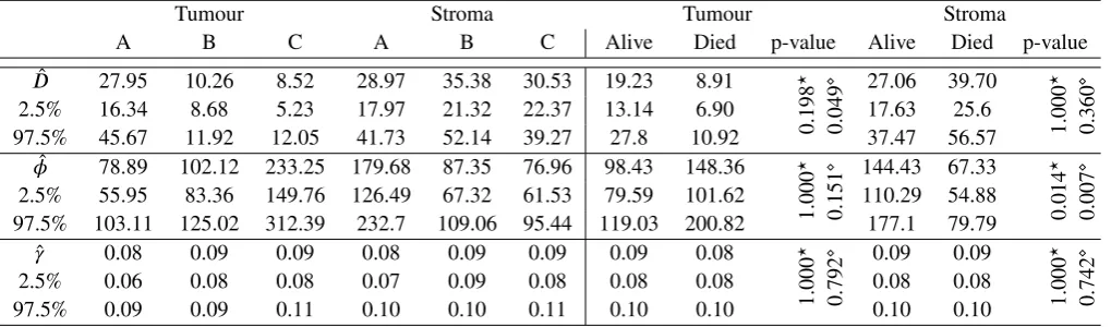
TABLE 2Summaries of the bootstrapped resamples for parameters of the Thomas process: summarised by the mean value and 95% confidence intervals for both tumour and stroma patterns at each Dukes grade, A, B, and C, and patient mortality at follow up, Alive or Died. The p-values relate to a permutation test as follows:𝐻₀ ∶|𝜇_{𝐷𝑖𝑒𝑑}−𝜇𝐴𝑙𝑖𝑣𝑒|= 0vs𝐻₁∶|𝜇_{𝐷𝑖𝑒𝑑}−𝜇𝐴𝑙𝑖𝑣𝑒|≠0. To adjust for multiple comparisons we use both the Bonferroni correction method and a false discovery rate correction.18These are denoted by the superscripts⋆and⋄respectively.

Tumour Stroma Tumour Stroma

A B C A B C Alive Died p-value Alive Died p-value

̂

𝐷 27.95 10.26 8.52 28.97 35.38 30.53 19.23 8.91

0

.

198

⋆

0

.

049

⋄ 27.06 39.70

1

.

000

⋆

0

.

360

⋄

2.5% 16.34 8.68 5.23 17.97 21.32 22.37 13.14 6.90 17.63 25.6

97.5% 45.67 11.92 12.05 41.73 52.14 39.27 27.8 10.92 37.47 56.57 ̂

𝜙 78.89 102.12 233.25 179.68 87.35 76.96 98.43 148.36

1

.

000

⋆

0

.

151

⋄ 144.43 67.33

0

.

014

⋆

0

.

007

⋄

2.5% 55.95 83.36 149.76 126.49 67.32 61.53 79.59 101.62 110.29 54.88

97.5% 103.11 125.02 312.39 232.7 109.06 95.44 119.03 200.82 177.1 79.79

̂𝛾 0.08 0.09 0.09 0.08 0.09 0.09 0.09 0.08

1

.

000

⋆

0

.

792

⋄ 0.09 0.09

1

.

000

⋆

0.742

⋄

2.5% 0.06 0.08 0.08 0.07 0.09 0.08 0.08 0.08 0.08 0.08

97.5% 0.09 0.09 0.11 0.10 0.10 0.11 0.10 0.10 0.10 0.10

Matérn process

The bootstrap resamples of the estimated Matérn process parameters for the tumour and stroma patterns are summarised in Table 3. The differences are similar to those noted above when assuming a Thomas cluster process. This is to be expected as both are cluster processes but differ only in their structure of a cluster.

The permutation test (using the false discovery rate correction) indicates that in respect of discriminating between patient mortality outcomes find that

(i) There is strong evidence (p-value 0.01) to suggest that stroma nuclei patterns of patients who died from CRC have on average a lower number of daughters per parent,𝜙̂. This is also indicated by the results of the Cox proportional hazards model where the hazard ratio was estimated as HR= 0.198, CI(0.053,0.740).

(ii) There is evidence (p-value 0.055) to suggest that tumour parent density,𝐷̂, is lower in patient’s who died from CRC. Using Cox proportional hazard the results also indicate that patients with lower (scaled) parent density are less likely to die, HR

= 0.388, CI(0.156,0.965).

These results again align with the patient’s Dukes grading. For example, stroma nuclei patterns of patients graded Dukes C had on average a lower daughter density than those graded Dukes A. The difference is less clear when considering patients graded Dukes B; this we might expect as Grade B patients were a mixture (∼ 50%) of patients who died from CRC and those still alive at follow up.

3.2

Assessing model fit using the empty space function

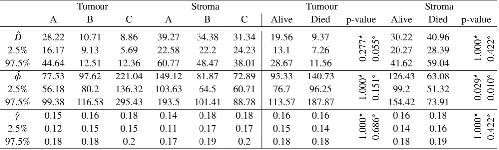
TABLE 3Summaries of the bootstrapped resamples for the Matérn process parameters: summarised by the mean value and 95% confidence intervals for both tumour and stroma patterns at each Dukes grade, A, B, and C, and patient mortality at follow up, Alive or Died. The p-values relate to a permutation test as follows:𝐻₀ ∶|𝜇𝐷𝑖𝑒𝑑−𝜇𝐴𝑙𝑖𝑣𝑒|= 0vs𝐻1∶|𝜇𝐷𝑖𝑒𝑑−𝜇𝐴𝑙𝑖𝑣𝑒|≠0. To adjust for multiple comparisons we use both the Bonferroni correction method and a false discovery rate correction.18_These are denoted by the superscripts⋆and⋄respectively.

Tumour Stroma Tumour Stroma

A B C A B C Alive Died p-value Alive Died p-value

̂

𝐷 28.22 10.71 8.86 39.27 34.38 31.34 19.56 9.37

0.277

⋆

0.055

⋄ 30.22 40.96

1.000

⋆

0.422

⋄

2.5% 16.17 9.13 5.69 22.58 22.2 24.23 13.1 7.26 20.27 28.39

97.5% 44.64 12.51 12.36 60.77 48.47 38.01 28.67 11.56 41.62 59.04 ̂

𝜙 77.53 97.62 221.04 149.12 81.87 72.89 95.33 140.73

1.000

⋆

0.151

⋄ 126.43 63.08

0.029

⋆

0.010

⋄

2.5% 56.18 80.2 136.32 103.63 64.5 60.71 76.7 96.25 99.2 51.32

97.5% 99.38 116.58 295.43 193.5 101.41 88.78 113.57 187.87 154.42 73.91

̂𝛾 0.15 0.16 0.18 0.14 0.18 0.18 0.16 0.16

1.000

⋆

0.686

⋄ 0.16 0.18

1.000

⋆

0.422

⋄

2.5% 0.12 0.15 0.15 0.11 0.17 0.17 0.15 0.14 0.14 0.16

97.5% 0.18 0.18 0.2 0.17 0.19 0.2 0.18 0.18 0.18 0.19

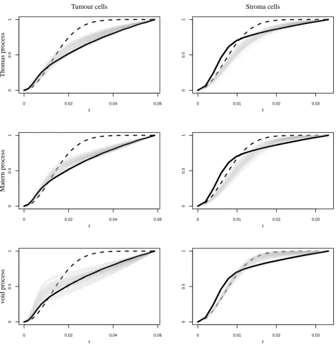
In order to informally assess the fit of the models to the CRC data we compare the spatial patterning of the observed data and the data simulated from the fitted model through using the estimated empty space function,𝐻(𝑟).12_{In two-dimensions, this} describes the probability that the disc𝑏(𝑥, 𝑟)of radius𝑟centered at𝑥is not empty. In the stationary case assumed here (i.e., shifting the pattern by a vector does not affect the distribution of points) the disc may be centered at the origin (i.e.,𝑏(𝑜, 𝑟)).

Figure 4 shows the empty space functions for each considered point process for the image shown in Figure 3. Solid lines represent the estimated empty space function for the fitted model. The grey dotted lines are the estimated empty space functions from patterns simulated with the parameter estimates from the fitted model (i.e., the estimated parameters for the set of images to which Figure 3 belongs). The empty space function is estimated using the Chiu-Stoyan estimator employed in theRpackage spatstat.20 _{The dashed lines are the theoretical empty space function for a homogeneous Poisson process,1 −exp(−𝜆𝜋𝑟}2₎

where𝜆is point density and𝑟is the interpoint distance.12

We assess the models fit in Figure 4 by looking for overlap between the envelope of the empty space functions for the simulated data, shown by the grey lines, and the empirical empty space function for the fitted model, shown by the solid line. Comparison of the solid line and the dashed line compares the fitted CRC model to a homogeneous Poisson process where the probability of points in a sphere of radius𝑟is proportional to the area of that sphere.

The overlap of the envelope of the empty space functions for the simulated data and the empirical empty space function for the fitted model shown in the left hand plots of Figure 4 indicate that the tumour pattern could be a realisation of either a Thomas, Matérn, or void process. The right hand top and middle rows of Figure 4 indicate that the pattern formed by stroma cells is slightly less likely to have nearby points at the same distances as a NSPP (either a Thomas or Matérn process).

From Figure 4 we see that the stroma cell pattern more quickly approaches that of a homogeneous Poisson process; this is the case at a distance of 3% of the width and height of the image (𝑟= 0.03). This seems reasonable from the pattern of stroma cells shown in Figure 3 and is also reflected by the estimated lower void density for stroma cells (Table 1), which would lead to a pattern with fewer gaps.

A comparison of the empty space function for both the tumour and stroma cell patterns to that of the homogeneous Poisson process (dashed lines) reveals that at short distances the cells exhibit some regularity, whereas only at longer distances does the pattern exhibit clustering. This is expected as in both cases the points represent cell nuclei, and due to the size of the cells at short distances no other cells (points) can exist.

4

DISCUSSION

sections by treating their nuclei locus as a spatial point pattern and consider three spatial point processes (void, Thomas, Matérn), taking a Palm likelihood approach for parameter estimation in each case. This estimation is nontrivial and is achieved through extending existing work10 _{which uses the interpoint distances between points (cells) to inform consideration of the spatial} morphology of the tissue structure.

We illustrate that by using estimated parameters of the Palm intensity function as classifiers of the spatial morphology of cancerous tissue sections that the patterns formed by cells may be informative as to CRC patient survival. Although no one model would perfectly encapsulate the intricacies in the spatial structure of this tissue, we believe our methods open the door to taking a more analytical approach to describe these types of data. Although beyond the scope of this work, other point process models could be used in this setting. For example, the pattern of all nuclei (tumour and stroma) could be considered to be a realisation of a marked point process with cell type as a mark (i.e., characteristic of the point). This approach would consider all cell nuclei to be realisations from the same spatial point process where characteristics of the points (marks i.e., cell type) were realisations of another process, which would encompass the inter- and intra- mark interactions. However, such an approach would presume that the mark process followed some defined formulation. Furthermore, using latent structures in a marked log-Gaussian Cox process, for example, might enable the mark-point dependence to be inferred. Yet, in this case, a dependence between cell types and their location is not likely and not of particular interest. In our work we fit models to each pattern (tumour and stroma) independently to capture the spatial spatial features exhibited in each.

The modelling framework detailed herein provides a standardised methodology that describes and reports the spatial distribu-tion of cells in cancerous tissue secdistribu-tions in a way that negates observer variability. That is, we do not rely human classificadistribu-tions of tissue morphology but use the pattern formed by the cells themselves to infer patterning in tissue structure. Using this method-ology we rely on the ability of the imaging software to, with negligible error, pinpoint locations of the cell nuclei and to correctly identify the type of cell (i.e., tumour or stroma). Our proposed framework indicates that certain parameters of the processes we discuss are useful indicators of patient mortality. These parameters also align with the different Dukes staging the tissue sam-ples were classified as by pathologists. This is not surprising as the grades were given by experts in the field and can be thought to roughly reflect the severity of the tumour; hence, they are a good indicator of patient outcome.

The literature reports morphological features such as tumour budding to be significantly associated with disease survival. However, the lack of consensus on quantification methods and observer variability has led to their exclusion from clinical guide-lines.21_{In brief, high tumour budding is found in patients with an infiltrative growth pattern: finger-like protrusions invading} widely across the stroma and thus forming large gaps between the cancer protrusions. Both tumour budding and infiltrative growth pattern would be reflective of the tumour cell void patterning described herein. In contrast, low tumour budding, or a pushing border growth pattern, described as a solid tumour mass with little stroma existing between cells, has been correlated with good outcome.22_{However cancerous tissue sections typically lack histopathological features that can be reliably identified} and reproducibly quantified by eye. Our work uses an analytical framework to identify potential indicators of patient survival without the need to rely human observation and risk potential bias.

More broadly, this work reflects a growing interest in the use of analytical techniques in recognition of the importance of both spatial structure and spatial variations within cellular data. For example, in some cases it was observed that both the abundance of immune cells and their spatial variation within the tumour are important factors in patient outcome.23_{In addition, a recent review} of spatial heterogeneity in cancers outlined the importance and relevance of spatial statistics in describing cellular patters.24 Here, we demonstrate that analytical methods perhaps more commonly used in ecological contexts10,15_{may be used and built} upon to aid understanding of the spatial structure of CRC tissue sections.

The methodology we describe above may be used to describe subjectively reported histopathological features such as infil-trative invasion pattern and tumour budding throughout the stroma. This is a known, and common, phenomenon that has been previously highly subjective and not reproducible through manual observation.******CITATION NEEDED PETER*******

ACKNOWLEDGEMENTS

0

0.5

1

0 0.02 0.04 0.06

r

Tumour cells

Thomas process

0

0.5

1

0 0.01 0.02 0.03

r

Stroma cells

0

0.5

1

0 0.02 0.04 0.06

r

Matern process

0

0.5

1

0 0.01 0.02 0.03

r

0

0.5

1

0 0.02 0.04 0.06

r

v

oid process

0

0.5

1

0 0.01 0.02 0.03

r

FIGURE 4This figure illustrates for one image of one patient’s slide, that shown in Figure 3, how the empty space function, H(r), can be used to informally asses the model fit in each instance of the Thomas, Matérn, and void process. The dashed black line in each panel shows H(r) for a homogeneous Poisson process (i.e., a constant intensity of points within some given region). We would expect H(r) for our point pattern of cells to deviate from this. This is indeed the case in each panel. The empty space function, H(r), for the tissue pattern is shown by the solid black line, which does deviate from the homogeneous Poisson line. The bottom right plot shows an overlap between the simulated pattern’s empty space function and that of the homogeneous Poisson process for the stroma nuclei. Looking again at Figure 3 this seems somewhat plausible as the stroma cells do seem to

“blanket” the image. In each plot the distance𝑟represent the percentage of the image’s width and height scaled to be∈ [0,1].

References

1. Mattfeldt T, Fleischer F. Characterization of squamous cell carcinomas of the head and neck using methods of spatial statistics.Journal of Microscopy2014; 256(1): 46–60.

2. Caie PD, Zhou Y, Turnbull AK, Oniscu A, Harrison DJ. Novel histopathologic feature identified through image analysis augments stage II colorectal cancer clinical reporting.Oncotarget2016; 7(28): 44381.

3. Pinheiro RS, Herman P, Lupinacci RM, et al. Tumor growth pattern as predictor of colorectal liver metastasis recurrence. The American Journal of Surgery2014; 207(4): 493–498.

4. Tokodai K, Narimatsu H, Nishida A, et al. Risk factors for recurrence in stage II/III colorectal cancer patients treated with curative surgery: the impact of postoperative tumor markers and an infiltrative growth pattern.Journal of surgical oncology 2016; 114(3): 368–374.

5. Morikawa T, Kuchiba A, Qian ZR, et al. Prognostic significance and molecular associations of tumor growth pattern in colorectal cancer.Annals of surgical oncology2012; 19(6): 1944–1953.

6. Rieger G, Koelzer VH, Dawson HE, et al. Comprehensive assessment of tumour budding on cytokeratin stains in colorectal cancer.Histopathology2017; 70(7): 1044–1051.

7. De Smedt L, Palmans S, Sagaert X. Tumour budding in colorectal cancer: what do we know and what can we do?.Virchows Archiv2016; 468(4): 397–408.

8. Caie PD, Turnbull AK, Farrington SM, Oniscu A, Harrison DJ. Quantification of tumour budding, lymphatic vessel density and invasion through image analysis in colorectal cancer.Journal of Translational Medicine2014; 12(156): 1–12.

9. Neyman J, Scott EL. Statistical approach to problems of cosmology.Journal of the Royal Statistical Society. Series B (Statistical Methodology)1958; 20(1): 1–43.

10. Stevenson BC, Borchers DL, Fewster RM. Cluster capture-recapture to account for identification uncertainty on aerial surveys of animal populations. In submission.

11. Tanaka U, Ogata Y, Stoyan D. Parameter Estimation and Model Selection for Neyman-Scott Point Processes.Biometrical Journal2008; 50(1): 43–57.

12. Illian J, Penttinen A, Stoyan H, Stoyan D.Statistical analysis and modelling of spatial point patterns. Chichester: John Wiley & Sons . 2008.

13. Coeurjolly JF, Møller J, Waagepetersen R. A tutorial on Palm distributions for spatial point processes. International Statistical Review2017; 85(3): 404–420.

14. Li S. Concise formulas for the area and volume of a hyperspherical cap.Asian Journal of Mathematics and Statistics2011; 4(1): 66–70.

15. Fewster RM, Stevenson BC, Borchers DL. Trace-contrast models for capture–recapture without capture histories.Statistical Science2016; 31(2): 245–258.

16. Tu SJ, Fischbach E. Random distance distribution for spherical objects: general theory and applications to physics.Journal of Physics A: Mathematical and General2002; 35(31): 6557.

17. Stevenson BC.palm: Fitting point process models using the Palm likelihood. 2017.

18. Benjamini Y, Hochberg Y. Controlling the false discovery rate: a practical and powerful approach to multiple testing.Journal of the royal statistical society. Series B (Methodological)1995; 57(1): 289–300.

20. Baddeley A, Rubak E, Turner R.Spatial Point Patterns: Methodology and Applications with R. London: Chapman and Hall/CRC Press . 2015.

21. Karamitopoulou E, Zlobec I, Koelzer VH, Langer R, Dawson H, Lugli A. Tumour border configuration in colorectal cancer: proposal for an alternative scoring system based on the percentage of infiltrating margin. Histopathology 2015; 67(4): 464–473.

22. Zlobec I, Baker K, Minoo P, Hayashi S, Terracciano L, Lugli A. Tumor border configuration added to TNM staging better stratifies stage II colorectal cancer patients into prognostic subgroups.Cancer2009; 115(17): 4021–4029.

23. Nawaz S, Heindl A, Koelble K, Yuan Y. Beyond immune density: critical role of spatial heterogeneity in estrogen receptor-negative breast cancer.Modern Pathology2015; 28: 766–777.

24. Heindl A, Nawaz S, Yuan Y. Mapping spatial heterogeneity in the tumor microenvironment: a new era for digital pathology. Laboratory Investigation2015; 95: 377–384.

APPENDIX

A THE PALM INTENSITY FUNCTION

This appendix derives the d-dimensional Palm intensity functions for both the void and Matérn processes, Section 2. The appli-cation, Section 3, considers only the 2-dimensional case; therefore, above, we only provide the details of the Palm intensities and likelihoods in 2-dimensions. In this appendix we generalise this to consider d-dimensions. Due to this we now consider, for example, the volume of hyperspheres, and not the area of circles.

A.1 A d-dimensional void point process

We define a𝑑-dimensional void process as follows. Let𝑋̄ and𝑃 be independent homogeneous Poisson processes on𝑅d_{. Then} the void process is given by𝑋 =𝑋̄∖(⋃_𝑝∈𝑃𝑏(𝑝, 𝑅)), where𝑏(𝑣, 𝑅) = {𝑢∈𝑅d ∶||𝑢−𝑝||≤𝑅}is the ball centered at v with radius𝑅 >0.

R

R

●

● ●

Rcos(θ) I(r) A(r)

R

r

R Rsin(θ)

θ ●

● ●

observed daughter potential daughter

parent doesn't delete potential daughter parent deletes potential daughter

i)

● _r ●

ii)

FIGURE A1Plot i) illustrates the geometry of the intersection,𝐼(𝑟) =𝑏(𝑑_𝑜, 𝑅) ∩𝑝(𝑑_𝑝, 𝑅), of two circles of radius𝑅centered at𝑑_𝑜and𝑑_𝑝

To calculate 𝐼(𝑟), in Figure A1, the integrand of the volume of a d− 1 sphere of radius𝑅sin(𝜽)with height 𝑅cos(𝜽)is required. As the hyperspheres are of common radius (𝑅being the radius of a void)𝐼(𝑟)is simply just twice this volume.14This is given by,

𝐼d(𝑟) = 2 ×

𝜙

∫

0

𝑣d−1(𝑅sin𝜽)d𝑅cos𝜽,

= 2 ×

𝜙

∫

0

𝑣d−1(𝑅sin𝜽)𝑅sin𝜽d𝜽,

= 2 × 𝜋

d−1 2

Γ(d−1

2 + 1)

𝑅d 𝜙

∫ 𝑜

sind𝜽d𝜽,

= 2 × 𝜋

d−1 2

Γ(d−1

2 + 1)

𝑅dJ_𝑑(𝜙),

= 𝜋

d−1 2

Γ(d−1

2 + 1)

𝑅d𝐵(d+ 1

2 ,

1 2

)

I(sin2𝜙;d+ 1

2 ,

1 2

) ,

=𝑣d(𝑅)I(sin2𝜙;d+ 1

2 ,

1 2

) ,

=𝑣d(𝑅)I (

1 −( 𝑟 2𝑅

)2

;d+ 1

2 , 1 2 ) , (A1)

noting that𝐵(𝑎, 𝑏) = Γ(𝑎) Γ(𝑏)

Γ(𝑎+𝑏) ,Γ

(₁

2

)

=√𝜋, and that(𝑅cos𝜽)2_{+ (𝑅sin𝜽)}2_=𝑅2_→(sin𝜽)2_{= 1 − (cos𝜽)}2_{and using the cosine}

rule leads to cos𝜽= 𝑟2+𝑅2−𝑅2

2𝑟 𝑅 =

𝑟

2𝑅. Here I(𝑧;𝑎, 𝑏) = 𝐵(𝑧;𝑎,𝑏)

𝐵(𝑎,𝑏) is the regularised Beta function.

Recall that the Palm intensity of the void process can be written as 𝜆₀(𝑟) = 𝜆 𝑝_𝑠(𝑟) where𝑝_𝑠(𝑟) = exp(−𝐷 𝐴(𝑟)) is the probability that an arbitrary point has no parent within a some distance 𝑅. Here 𝐴(𝑟) = 𝑣d_{(𝑅) −𝐼(𝑟)where 𝑣}d_{(𝑅) is the} d-dimensional volume of a hypershpere of radius𝑅. Then the Palm intensity is given by

𝜆₀(𝑟) =𝜆exp (

−𝐷 𝑣d(𝑅)

[

1 −I (

1 −( 𝑟 2𝑅

)2

;d+ 1

2 ,

1 2

)]) ,

=𝜆exp(−𝐷 𝑣d(𝑅)[1 −F_𝑔(𝑟)(d+ 1

2 , 1 2 )]) , (A2)

where𝑔(𝑟) = 1 −( 𝑟

2𝑅

)2

, and F_𝑔(𝑟)(⋅,⋅)is the CDF of the Beta distribution. Thus, when𝑟 = 0⇒𝑔(𝑟) = 1⇒F₁(⋅,⋅) = 1⇒

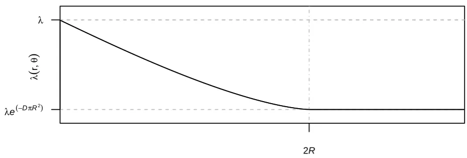
𝜆₀(0) = 𝜆. In addition, when𝑟 = 2𝑅⇒𝑔(𝑟) = 0⇒F₀(⋅,⋅) = 0⇒𝜆₀(0) = 𝜆exp(−𝐷 𝑣d(𝑅)), due to the properties of the CDF. The functional form of this Palm intensity is shown in Figure A2. Letting d= 2in Equation (A2) would lead to the Palm intensity given in Equation (2).

A.2 A d-dimensional Matérn point process

λ

(

)

λe(−DπR2) λ

FIGURE A2 The functional form of the Palm intensity for the void process in 2 dimensions. The horizontal asymptote is given by

𝜆exp(−𝐷𝜋𝑅2_{), which is the value that𝜆}

0(𝑟)decays to for values of𝑟 ≥2𝑅. The Palm intensity at𝑟= 0is simply𝜆, as for𝑟= 0𝑔(𝑟) = 1

in Equation 2, thus the exponential becomes1. At the value𝑟 = 2𝑅the volume of intersection between the spheres encircling an observed daughter and a potential point of radius𝑅is zero, thus the contribution from the CDF of the Beta distribution to𝜆(𝑟;𝜃)is zero.

The d-dimensional version of Equation 6 is given by,

𝑓_𝑦d(𝑟;𝛾) = 2d

𝐵(d

2 +

1 2,

1 2)

𝑟d−1 𝛾d+1

[

2𝐹1

(₁ 2, 1 2− d 2, 3 2,1

) 𝛾−₂𝐹₁

( 1 2, 1 2− d 2, 3 2, 𝑟2

4𝛾2

) 𝑟 2 ] , =

2d𝑟d−1 _∫𝛾 𝑟 2

(𝛾2_−𝑥2₎d−12 𝑑𝑥

𝐵(d

2+

1 2,

1 2)𝛾

2d .

(A3)

Here𝐵(⋅,⋅)denotes the beta function, and₂𝐹₁(⋅,⋅,⋅,⋅)the hyper-geometric function.

Below we show how this PDF reduces in𝑑 = 2and𝑑 = 3to forms equivalent to the PDFs of the distances between two randomly selected sisters in the respective dimensions.12, p.376

∙for d= 2It should be noted that,

𝛾

∫

𝑟 2

(𝛾2−𝑥2)d−12 𝑑𝑥=

𝛾

∫

𝑟 2

(𝛾2−𝑥2)12𝑑𝑥

= 1

8

(

4𝛾2sec−1 (

2𝛾 𝑟

)

−𝑟√4𝛾2_−𝑟2

) .

therefore,

2d𝑟d−1 _∫𝛾 𝑟 2

(𝛾2_−𝑥2₎d−12 𝑑𝑥

𝐵(d

2+

1 2,

1 2)𝛾

2d =

4𝑟∫𝑟𝛾 2

(𝛾2_−𝑥2₎12𝑑𝑥

𝐵(3

2, 1 2)𝛾

4

= 𝑟Γ(2)

1 2

√ 𝜋2𝛾4₂

(

4𝛾2sec−1 (

2𝛾 𝑟

)

−𝑟√4𝛾2_−𝑟2

)

= 𝑟

𝜋 𝛾4

(

4𝛾2sec−1 (

2𝛾 𝑟

)

−𝑟√4𝛾2_−𝑟2

)

= 𝑟

𝜋 𝛾4

(

4𝛾2cos−1 (

𝑟

2𝛾 )

−𝑟√4𝛾2_−𝑟2

) ,

noting that sec−1_{(𝑥) =cos}−1(1

𝑥 )

, and as𝐵(3

2, 1 2) =

Γ(3₂) Γ(1₂)

Γ(2) , recalling thatΓ( 3 2) =

1 2

√ 𝜋,Γ(1

2) =

√

∙for d= 3It should be noted that, 𝛾

∫

𝑟 2

(𝛾2−𝑥2)d−12 𝑑𝑥=

𝛾

∫

𝑟 2

(𝛾2−𝑥2)𝑑𝑥

= 1

24 (𝑟− 2𝛾)

2 _{(𝑟+ 4𝛾).}

therefore,

2d𝑟d−1 ∫𝑟𝛾 2

(𝛾2−𝑥2)d−12 𝑑𝑥

𝐵(d

2+

1 2,

1 2)𝛾

2d =

6𝑟2 ∫𝑟𝛾 2

(𝛾2−𝑥2)𝑑𝑥

𝐵(2,1

2)𝛾 6

= 6𝑟2

24𝐵(2,1

2)𝛾

6 (𝑟− 2𝛾) 2

(𝑟+ 4𝛾),

=

𝑟2_Γ(5 2)

4𝛾6_{Γ(2) Γ(}1 2)

(𝑟− 2𝛾)2 (𝑟+ 4𝛾)

=

𝑟2 3

4

√ 𝜋

4𝛾6√_𝜋 (𝑟− 2𝛾)

2 _{(𝑟+ 4𝛾)}

= 3𝑟

2

16𝛾6 (𝑟− 2𝛾)

2 _{(𝑟+ 4𝛾)}

= 3𝑟

2

16𝛾6

( 𝛾− 𝑟

2

)2(

2𝛾+ 𝑟 2

) .

noting thatΓ(5

2) = 3 4

√ 𝜋,Γ(1

2) =

√

𝜋, andΓ(2) = 1.

Upon substitution of the PDF (Equation A3) into the Palm intensity function (Equation 3) simplifications occur—this is also the case for the modified Thomas process, Section 2.3.10_{These simplifications circumvent the numerical instability in𝜆(𝑟;𝜽)} at𝑟= 0as both the numerator and denominator in the second term contain the term𝑟𝑑−1. Thus,

𝜆(𝑟;𝜽) =𝐷 𝐸_𝑐(𝜙) +[

𝐸_𝑠(𝜙) − 1]𝑓d 𝑦(𝑟;𝛾) 𝑠d_(𝑟) ,

=𝐷 𝐸_𝑐(𝜙) +[𝐸𝑠(𝜙) − 1] 2d

𝐵(d

2+

1 2,

1 2)

𝑟d−1

𝛾d+1

Γ(d

2 + 1)

d𝜋𝑑∕2_𝑟d−1

×

[

2𝐹1

(₁ 2, 1 2− d 2, 3 2,1

) 𝛾−₂𝐹₁

( 1 2, 1 2− d 2, 3 2, 𝑟2

4𝛾2

) 𝑟

2

] ,

=𝐷 𝐸_𝑐(𝜙) + 2 [𝐸𝑠(𝜙) − 1]

𝐵(d

2+

1 2,

1 2)𝛾

d+1

Γ(d

2+ 1)

𝜋𝑑∕2

×

[

2𝐹1

(₁ 2, 1 2− d 2, 3 2,1

) 𝛾−₂𝐹₁

( 1 2, 1 2− d 2, 3 2, 𝑟2

4𝛾2

) 𝑟

2

] ,

=𝐷 𝐸_𝑐(𝜙) +2 [𝐸𝑠(𝜙) − 1]

𝛾d+1_𝜋d2

Γ(d

2 + 1)

2

Γ(d

2+

1 2) Γ(

1 2)

×

[

2𝐹1

(₁ 2, 1 2− d 2, 3 2,1

) 𝛾−₂𝐹₁

( 1 2, 1 2− d 2, 3 2, 𝑟2

4𝛾2

) 𝑟

2

] ,

=𝐷 𝐸_𝑐(𝜙) +2 [𝐸𝑠(𝜙) − 1]

𝛾d+1_𝜋12(d+1) Γ(d

2+ 1) 2 Γ(d 2+ 1 2) × [

2𝐹1

(₁ 2, 1 2− d 2, 3 2,1

) 𝛾−₂𝐹₁

( 1 2, 1 2− d 2, 3 2, 𝑟2

4𝛾2

) 𝑟 2 ] . (A4)

noting that𝐵(𝑥, 𝑦) = Γ(𝑥) Γ(𝑦)

Γ(𝑥+𝑦) , andΓ( 1 2) =