Robust Estimation of the Normal Distribution Parameters by Use of Structural Partitioning Perobls D Method

(1)

https://www.scirp.org/journal/ajcm ISSN Online: 2161-1211

ISSN Print: 2161-1203

DOI: 10.4236/ajcm.2019.94022 Dec. 17, 2019 302 American Journal of Computational Mathematics

Robust Estimation of the Normal-Distribution

Parameters by Use of Structural

Partitioning-Perobls D Method

Gligorije Perović

Department of Geodesy and Geoinformatics, Faculty of Civil Engineering, University of Belgrade, Belgrade, Serbia

Abstract

Quite many authors have dealt with the estimation of the parameters of nor-mal distribution on the basis of non-homogeneous sets: Hald A. 1949 [1], Arango-Castillo L. and Takahara G. 2018 [2]. All the robust methods are based on the assumption that the results affected by gross errors can be found to the left and/or to the right of censoring, or truncated, points. However, as a rule, the (intrinsic) distribution of observations is complex (mixed) consisting of two or more distributions. Then the existing methods, such as ML, Huber’s, etc., yield enlarged estimates for the normal-distribution variance. By study-ing better estimates the present author has invented new method, called PEROBLS D, based on the Tukeyan mixed-distribution model in which both the contamination rate (percentage) and the parameters of both distributions, forming the mixed one, are estimated, and for the parameters of the basic normal distribution better estimates are obtained than by the existing me-thods.

Keywords

Non-Homogeneous Sets of Observations, Tukeyan Mixed-Distributions, Robust Perobls D Method

1. Introduction and History of Robust Estimation

The history of this problem is older than 300 years. For example, Galileo as long ago as in 1632 used the least absolute sum in order to reduce the effect of obser-vational errors to the estimate of the measured quantity [3], whereas Rudjer Boscovich, is the first who, as early as in1757, rejected clearly outlying observa-tions [4], also done by Daniel Bernouli 1777 [4]. The trimmed mean has been

How to cite this paper: Perović, G. (2019) Robust Estimation of the Normal-Distribu- tion Parameters by Use of Structural Parti-tioning-Perobls D Method. American Journal of Computational Mathematics, 9, 302-316. https://doi.org/10.4236/ajcm.2019.94022

Received: September 3, 2019 Accepted: December 14, 2019 Published: December 17, 2019 Copyright © 2019 by author(s) and Scientific Research Publishing Inc. This work is licensed under the Creative Commons Attribution International License (CC BY 4.0).

http://creativecommons.org/licenses/by/4.0/

(2)

DOI: 10.4236/ajcm.2019.94022 303 American Journal of Computational Mathematics

used since long ago, see “Anonymous” 1821 [4]. The first formal rules for re-jecting of observations were proposed by Peirce 1852 and Chauvenet 1863, and somewhat later appear the papers by Stone 1868, Wright 1884, Irvin 1925, Stu-dent 1927, Thompson 1935, and by many others [4].

The mixed distribution models have been also considered since long ago:

Glaisher 1872/1873, Stone 1873, Edgeworth 1883, Newcomb 1886, Jeffreys 1932/ 1939 [4]. Tukey in 1960 [5] defined a mixed model as a mixture of two normal distributions of a basic Φ_

(

x−θ σ

)

_ and of a contaminating Φ_

(

x−θ

)

3σ_

distribution:

( ) (

1

) (

)

(

)

3

F x = − Φε _ x−θ σ_+ Φε _ x−θ σ_,

where

( )

1

(

2

)

exp 2 d 2

x

x _−∞ t t

Φ = −

π

∫

is the function of the standard normal

distribution. Here the elements of the contaminating set appear with probability

ε_{, (Tukey assumes}ε_{as a small number, about 5%), and behave as}_gross

er-rors. In this way the real distributions are represented through a normal-distribution model with weighted tails.

The term robustness began to be used since 1953 (introduced by G. E. P. Box) in order to discriminate the class of statistical procedures with little sensitivity to minor deviations from the starting assumptions. Some authors use the term sta-bility, but it is less used than the term robustness. In the Foreword of his book

ROBUST STATISTICS, Huber in 1981 [6] emphasizes that among the leading scientists in the late XIX and the early XX centuries there were a few statisticians —practitioners (and mentions: astronomer Newcomb, astrophysicist Eddington

and geophysicist Jeffreys) who expressed in their studies a perfectly clear under-standing of the robustness idea. They were aware of the perils caused by long tails of the functions of error distributions, so they proposed models of distribu-tion of gross errors and derived robust variants of standard estimates. Russian geodesists, for example, in their adjustments of the first order triangulation net-works allowed lower weights (about half of the original ones) to the observations of directions which do not deviate much.

The initial fundaments to the theory of robust estimation were laid by Swiss mathematician P. J. Huber 1964 [1] and American statistician W. J. Tukey 1960

[5]. Huber’s article “Robust Estimation of Location Parameter” was the first fundament of the theory of robust estimation, which introduced an elastic class of estimates, called M-estimates, which have become a very useful instrument, having established which properties they have (for instance consistency and asymptotic normality). He introduced the model of gross errors, replacing the strict parametric model F x

(

−θ

)

, with its known distribution F, by the mixed

model:

(

) (

1

) (

)

(

)

H x−θ = −ε F x−θ +εG x−θ ,

while a part of data ε (0≤ <

ε

1) may contain gross errors which have an

(3)

The causes of deviating from the parametric models are various and four main types of deviating from the strict parametric models can be distinguished:

1) Appearance of gross errors; 2) Rounding and grouping;

3) Using an approximate functional mode; and 4) Using an approximate stochastic model.

The fundamentals of robust methods were developed in the last century. To-day there are numerous applications of robust methods, and concurrently better and more detailed solutions are sought: [2][7]-[14].

Due to good properties of the robust methods—that it is possible to eliminate or decrease the influences of gross errors and outliers on the estimates of distri-bution parameters, in practice they are used more and more. Therefore, the same time, their development results. So the current development and application of the robust methods may be classified into the following groups:

Improvement of existing methods, such as “A new Perspective on Robust M. Estimation” [13];

Solving of delicate (specific) tasks:—for robust hybrid state estimation with unknown measurement noise statistics [14]—for optimal allocation of shares in a financial portfolio [8]—for robust estimation of 3D human poses from a single image [12]—for cubature Kalman filter for dynamic state estimation of synchronous machines under unknown measurement noise statistics [9];

Applications in various conditions:—for robust estimation of the sample mean variance for Gaussian processes with long-range dependence [2]—for robust estimation of 3D human poses from a single image [12]—for robust hybrid state estimation with unknown measurement noise [14]—for estima-tion of mean and variance using environmental data sets with below detec-tion limit observadetec-tions [10];

Applications in diverse fields:—for estimation of the sample mean variance for Gaussian processes with long-range dependence [2]—for Gaussian sum filtering with unknown noise statistics: Application to target tracking [11]

—robust cubature Kalman filter for dynamic state estimation of synchronous machines under unknown measurement noise statistics [9]—for estimation of mean and variance in Fisheries [7]—for optimal allocation of shares in a financial portfolio [8]—for estimation of mean and variance using environ-mental data sets with below detection limit observations [10].

The proposed PEROBLS D method is aimed at eliminating the influences of gross errors and outliers on the estimates of distribution parameters, when only one contaminating distribution is present, i.e. in the case of Tukey’s mixed dis-tribution.

(4)

value and then the parameters of both distributions are estimated.

Consequently, in the case that both distributions (basic and contaminating) are normal, the PEROBLS D method has the following properties:

1) Unbiased (exact) parameter estimates for the basic distribution, as the most important property;

2) Unbiased (exact) parameter estimates for the contaminating distribution; 3) Percentage estimates for fractions of basic and contaminating distributions in the mixed one.

The correctness of the method has been verified on exact (expected) values of some quantities from the mixed Tukeyan distribution, as well as on an example of simulated data for 200 measurements of one quantity.

Besides, the estimates of the mean and variance for the basic distribution have been compared with the same ones obtained by ML method, and the estimate basic distribution standard has been also compared with Tukey mad standard estimate.

As has been said, the PEROBLS D estimates are unbiased, whereas the esti-mates of the basic distriburion standard in both cases, according to ML and Tu-key mad, are increased.

The structure of the further presentation is the following. At first definitions and notations are given, then basis of PEROBLS D method and the way of solv-ing the formulated problem. Afterwards the existsolv-ing robust estimation methods —ML and Huber’s mad—are presented. Further on the PEROBLS D method is verified on examples and the solutions are compared with existing ones. Finally, there are conclusions and references.

2. Definitions and Notations

The density function for a standard normal variable Z is given as

( )

1 _exp

(

2 ₂

)

2

f z = −z

π , −∞ < < ∞z .

Let F z

( )

be the notation of the distribution function for Z. The quintiles of

Z will be denoted as z1−α, where α is the significance level, zα = −z1−α and

(

1

)

(

1

)

1

p Z≤z₋_α =F z₋_α = −α.

A normally distributed r. v. X with expectation

µ

and variance

σ

2_{has the}

)

z= x−µ σ. (1)

Let as consider a random variable (natural sequence of measurements) [15]:

1, 2, , n

X X  X , from a normal population and use N

(

µ σ, 2

)

, with mean

µ

and standard deviation σ , (i.e. variance

σ

2_{) where one assumes that the}

ob-servations X X1, 2,,Xn are mutually independent. Arranging them in the

(5)

(Figure 1), where the points A and B defined in the following way:

(nX 1) 0.5

A=X ₊ − d and ₍ ₎ 0.5

Z

n n

B= X ₋ + d, (2)

where d is the width of the rounding interval for observations X. With z from Equation (1), it will be analogously:

( )1 ( )2 ( )X  ( X 1) ( Z) ( Z 1) ( )

A B

n n n n n n n

z z

Z ≤Z ≤≤Z ↓Z ₊ ≤≤Z ₋ ↓≤Z ₋ ₊ ≤≤Z ,

( )nX A (nX 1)

A

Z z µ Z

σ +

−

 

<_ = _≤

  ; (n nZ) B (n nZ 1)

B

Z z µ Z

σ

− − +

−

 

≤_ = _<

  ,

where z( )i =

(

x( )i −µ σ

)

.

3. Basis of PEROBLS D Method

1

The idea of PEROBLS D method has been presented in the Least Squares book

[16].

Instead of assuming the presence of gross errors in the observations within X

and Z regions, used in the previous methods, in this method the observation distribution is definedby means of Tukeyan mixed distribution (Figure 2):

( ) (

1

) ( )

1 2

( )

( ) ( )

(

)

(

) (

)

{

( ) ( )

(

)

(

)

(

₍ ₎ _{( )}

)

}

1

1 1 ,

X

X Z Z

A B n

n

A

n n B n n n

D D z z z z z

D D z z D D

′′

′ + ′ ′− ′′ ′− + ′′

′′ ∧ ∧ ′′ ∧ ′≤ ′ ∧ ′′≤ ′′≤ ′′

′ ′ ′ ′ ′′ ′′

∧ ∧ ∧ ∧ > ∧ ∧ ∧



 

where D( )′′1 =

(

X( )′′1 ≤ X′′≤ X( )′′1 +dx′′

)

, D( )′1 =

(

X( )′1 ≤X′≤X( )′1 +dx′

)

, , etc.

1_{PEROBLS D is an abbreviation of the initial letters: Perović’s Robust Least-Square Method; D—by}

(6)

[image:6.595.222.540.66.297.2]

[image:6.595.205.537.361.672.2]

Figure 1.Partition points, A and B.

Figure 2. Tukeyan mixed distribution of normally distributed

ob-servations.

Table 1. Designations and terms of the quantities appearing in the basic and the

contami-nating distributions.

Designations

Terms o f Quantities Basic Distribution Contaminating Distribution

X′ X′′ Random variable (observation)

1

σ σ2 Standard deviation (σ2>σ1)

µ µ _Expectation

n′ n′′ Number of measurements (total)

X

n′ n_X′′ Number of measurements in X region

Y

n′ nY′′ Number of measurements in Y region Z

n′ n_Z′′ _{Number of measurements in Z region}

Let

1 1 1

2 2 2

, ,

B

B A

A

x A B

z z z

x A B

z z z

µ

σ

µ

σ

′ − − − 

′= ′ = ′ =

 

′′ − − _{− }

′′= ′′= ′′=



(4)

( )

1 _exp

(

2 ₂

)

2

f z′ = z′

π ,

( )

(

)

2

1

exp 2 2

f z′′ = z′′

π .

Then the likelihood function, up to the proportionality constant k, is:

( )

(

) (

)

( )

(

)

( )

_{( )} 1 Y 2 X Z,

A B i

X

n n n

i i

Y Z

A B

L k f z p z z p z z z

f z p z z f z σ−′′ σ−′′− ′′

′′ ′ ′ ′′ ′′ ′′

= ⋅ ⋅ ≤ ⋅ ≤ ≤

′ ′ ′ ′′

⋅ ⋅ > ⋅ ⋅ ⋅

∏

[image:6.595.206.540.370.640.2]

(7)

where X, Y and Z under product sign mean:

( )

( ) 1

( )

X

n

i i

X f z′′ = i= f z′′

∏

, etc., and

where:

d ,

( )

d ,

A B

z z

X Y _z Z _z

d ,

A B

z z

X Y _z Z _z

A′′ =

∫

_−∞′′ z f z′′ ′′ z′′ A′′=

∫

_′′′′z f z′′ ′′ z′′ A′′=

∫

∞_′′z f z′′ ′′ z′′

( )

2 2 2

d , d , B d ,

A A

B

z z

X Z _z Y _z

B′ =

∫

_−∞′ z′ f z′ z′ B′ =

∫

∞_′ z′ f z′ z′ B′ =

∫

_′′′′z′′ f z′′ z′′

( )

, _B

( ) (

1 _B

)

,

A A A B

a′ = f z′ F′ b′ = f z′ −F′

( )

(

)

(

)

,

)

(

)

, , 1 ,

X A Y B A Z B

n′ =n F′ ′ n′ =n F′ ′−F′ n′ =n′ −F′

(

)

,

(

)

,

, 1

X A Y B A Z B

n′′ =n F′′ ′′ n′′=n′′ F′′−F′′ n′′=n′′ −F′′

then the conditions lnL 0

µ ∂

=

∂ , ₁

ln 0

L σ

∂ ₌

∂ and ₂

ln 0

L σ

∂ ₌

∂ yield the equations:

1 1 1 2 2 2

2

1 1 1 1 1

2 2

2 2 2 2 2

ln 1 1 1

0

ln 1

0

ln 1 1

0

A i i i

A

X Z Y

B Y AB X Z

Y X Z

A B Y i

X Z Y

AB i i

B

X Z

n n n

L

a b z d z z

n n n

L

z a z b z

n n n

L

g z z

µ σ σ σ σ σ σ

σ σ σ σ σ

′ ′ ′′  − ∂ _′ _′ _′ _′′ _′′ _′′ = + + − + + _{= } ∂ _  ′ ′ ′ − ∂ ₌ ₋ _{′ ′} ₊ _{′ ′}₊ _′ ₌   ∂ _  ′′ + ′′ ′′ ∂ _′′ _′′ _′′ = − − + + =  ∂ _

∑

(5)

solvable only iteratively. There are many methods; here direct iterations are giv-en.

However, within system (5), except

µ

,

σ

1 and

σ

2, the sums

∑

Yzi′,

i Xz′′

∑

,

∑

Zzi′′,

2 i Xz′′

∑

and 2

i Zz′′

∑

, and the numbers n′ and n′′ are also

unknown and they should be previously determined.

For the purpose of determining n′ and n′′ there are many ways. The present

author has examined a few methods out of which he has adopted the least-square one. With three relationships:

A B

A X X

B XY XY n

F n F n n v

n n n v

′ ′+ ′′ ′′= +   ′ ′+ ′′ ′′= + _  ′+ ′′= + _ (6)

where v_X,v_XY and v_n are the corrections to the “observations” n_X,n_XY and

(8)

1, 1

X XY

P = P = and Pn =1, we find the LS estimates for n′ and n′′:

(

)

1

n PU NV

D

= − _, n₂ 1

(

MV NU

)

D

= − _{, with}

(

)

(

)

2 2 2

2 2 1 , 1 1 , , A B

A B B B X A X Y B A B X A X Y B

M F F D MP N

N F F F F U n n F n n F

P F F V n n F n n F

 ′ ′ = + + = −  ′ ′ ′ ′′ ′ ′ = + + = + + + _  ′′ ′′ ′′ ′′ = + + = + + + _ and then 1

n′ =qn and n′′ =qn2 with

1 2 n q n n = + .

In this way the condition n′+n′′=n is satisfied, but the conditions:

X X X

n′ +n′′ =n , nY′ +nY′′=nY and nZ′ +nZ′′ =nZ are not satisfied. However, since

all conditions in Equations (6) cannot be satisfied simultaneously, a compromise yielding a solution close to the optimum must be accepted.

The sums

∑

(

)

2

i i

Z X′′−µ = Z X −µ − Z Xi′−µ

∑

,

and then by means the asymptotic theory according to which:

( )

1

( )

1

d d d

n n i

p i

X x f x x z f z z f z z

n µ σ µ

∞ ∞ ∞

′

′→∞

= ′→ = −∞ ′ ′ ′= −∞ ′ ′ ′+ −∞ ′ ′

′

∑

∫

,

(

)

2 2

(

) ( )

2 2 2

( )

1 1 1 1 d d n i n i p

X x f x x z f z z

n µ σ µ σ

∞ ∞

′

′→∞

= ′− → −∞ ′− ′ ′= −∞ ′ ′ ′

′

∑

∫

,

etc., it follows:

( )

1 d d

Y Y

n

Y Y Y

A p

i

F

X _′→∞ n

σ

z f z z n

µ

f z z

′ ′

′→ ′ ′ ′ ′+ ′ ′ ′

∑

∫

____

∫

__,

(

)

2 2 2

( )

1 d Y n Y Y B p i

X µ _′→∞ nσ z f z z

′

′− → ′ ′ ′ ′

∑

∫

_{},

one introduces the substitutions:

2

, , ,

i X i Z

Xz′′=n A′′ ′′ Zz′′=n A′′ ′′ Yxi′′=n′′σ AY′′+n′′µFY′′

∑

(

)

2

(

)

2

2 2 2 2 1 1 ,

i i Y Y Y

Yz′ =_σ  Y X −X +n X −µ −n′′σ BY′′

∑

(

)

2

(

)

2

2 2 1 2 2 1 , , .

i i D D D D

Dz σ D X X n X µ nσ B D X Y

 

′′ = _ − + − − ′ ′_ =

 

∑

where:

, , 1 .

X A Y B A Z B

F′′=F′′ F′′=F′′−F′′ F′′= −F′′

(9)

(

)

(

)

1 2, , 1, , , , ,

2 1, , , , , 2 2, 1 ,

k Y i k Y k k Z k B k X k A k

Y

k

X k X k Y k AB k

k

k k

k

X n A n b n a

n

n A n A n d

µ σ σ

σ σ +  _′′ _′′ _{′ ′} _′ _′ = _ − + −   ′′ ′′ ′′ ′′ ′′ ′′ + + −  

∑

(7)

(

)

2

(

)

2

2 2

1, 1 1 1, , , ,

,

2 2

1, , , , 2, ,

1

,

k Y i Y Y Y k k X k A k A k Y k

k Z k Bk B k k k Y k

X n n Z a

n

n Z b

X

n X

B

σ µ σ

σ σ + = _′  − + − + − ′ ′ ′  ′ ′ ′ ′′ ′′ + − _

∑

(8)

(

)

(

)

(

)

(

)

(

)

2 2 2

2

2, 1 1

, ,

2 ₂ ₂

1 2, , , 1, , ,

1

, k X i X Z i Z X X k

X k Z k

Z Z k k Y k AB k k k X k k Z k

X X n

n n

n n g n B n B

X X X

X

σ µ

µ σ σ

+ + +  = _ − + − + − ′′ + ′′  ′′ ′′ ′ ′ ′ ′ + − − + + _

∑

(9)

where: X 1 X i

X

X X

n

=

∑

_, _Y 1 _i

Y Y

X X

n

=

∑

_, _Z 1 _i

Z Z

X X

n

=

∑

_.

Let T 2 2

1, 2,

k = µk σ k σ k

x be the vector of parameter estimates in the k-th

iteration and dthe difference vector of these estimates from (k+1)-th and k-th iterations, then the iterations should be stopped if

{

}

10 q , 5, 6, 7,8, 9 .

k q

−

< ∈

d x

The points of optimal partition, Aopt and Bopt, with Aopt− = −µ

(

Bopt−µ

)

, are found from the condition

(

1−ε

) ( )

f x′ =εf x

( )

′′ , where 1− =

ε

n n′ and

n n

ε

= ′′ _{. So one obtains:}

(

2 1

)

2 2 1 2 2 ln , , . 1 1 opt opt n n

A µ A B µ A A σ σ

σ σ

′ ′′

′ ′ ′

= − = + =

− (10)

The advantagesof the method are: 1) Unbiased estimators for

µ

, 2

1

σ and 2

2

σ , if assumptions (4) hold and A

and B are close to Aopt and Bopt; and

2) Minimal variances for

µ

, 2 1

σ .

The disadvantagesof the method are:

1) A high sensitivity to the choice of the points A and B, (points A and B must be close to Aopt and Bopt), which can result in negative estimates for either of

the variances 2 1

σ or 2

2

σ , or for both; and

2) Sensitivity to the choice of the initial values for the variances 2 1

σ _and 2

2

σ _,

which, also, can result in negative estimates for one or both variances.

Therefore, the method is recommendable for applications comprising a high number of observations, (for example n>30).

Note 2. If there exists the basic distribution only (when in Equation (3)

ε

=0),

the method will yield either 2 2

1 2

σ =σ _{or negative values for one or both variances}_.

5. Some Robust Estimation

(10)

5.1. The Maximum Likelihood (ML) Method

The ML method is based on the assumption that in the domain Y there exists only the basic distribution, unlike the domaines X and Z where in addition to the basic distribution there exist gross errors and outliers. Here the censoring points are A and B and they are defined according to Equation (2).

In the region (X∪Z), due to the presence of gross errors in the observations,

the distribution of the random variable X is not normal. Therefore, the estimates of the parameters

µ

_{, and}

σ

2_{are determined on the basis of the probability of}

the event:

(

)

₍ ₎ ₍ ₎

(

)

{

X ≤ A ∧DnX+1 ∧ ∧ Dn n−Z ∧ B≤X

}

,

where the events Di=

{

Xi≤X ≤ Xi+dx

}

, i=nX +1,,n n− Z, mean that the

random variable X is within an interval

(

X X_i, _i+dx

)

(with differentially small dx>0).

Then the likelihood function, up to the proportionality constant, is [18]:

( )

_{( )}

( )

1 ! 1 ! !

X Z Z

X Z

X

n n n n

n n n

A i n i B

X Z

n

L F Z f z F Z

n n σ

− − − −

= +

= _ _

∏

_ − _ ,

and the ML estimators are the solutions of the equations

ln 0 L µ ∂ = ∂ , ln 0 L σ ∂ = ∂ . ln 0 L µ ∂ =

∂ , and

ln 0 L σ ∂ =

∂ . (11)

Equations (11) have no analytical solution and they must be solved iteratively.

There are several methods; here direct iterations are given:

( )

1 1 k k X Z

k k k

Y k Y k

f a f b

n n

n F

X

a n F b

µ ₊ = −σ ⋅ +σ ⋅

− , (12)

(

)

2

_{( )}

( )

_{( )}

2 2 2 2

1 1

1 k k k k

X Z

k k k k

Y k Y k

a f a b f b

n n

m

n F a F

X

n b

σ + = + −µ+ − ⋅σ + ⋅σ ₋ , (13)

where:

( )

(

)

2

2 1 1 1 1 , , Z Z X X

n n n n

i i

n n

Y Y

X m

n n

X =

∑

−₊ =

∑

−₊ X −X

, , k k k k k k A B a b a a µ µ − − = =

As initial values we can adopt

µ

0=X, and

2 2

0 m

σ = .

In the present author’s opinion under the preposition of existing of contami-nating distribution the method yields increased estimates for

σ

2_.

5.2. Huber’s Mad Robust Estimation of Distribution Standard

For the purpose of estimating an unknown standard σ Huber 1981 [6] and Birch and Mayers 1982 [17] proposed a median estimator for σ:

( )

0.6745

mad X

(11)

6. Results and Discussion

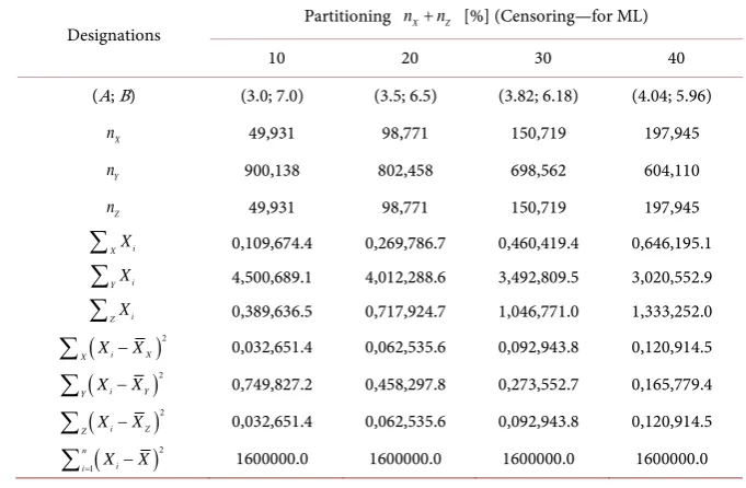
Example 1. For the sake of verifying the correctness of PEROBLS Dmethod and examining the appropriateness of Maximum Likelihood (ML) method in Table 2 are presented the exact (expected) values of some quantities from the mixed

Tukeyan distribution (3), with n′ =0.8n, n′′ =0.2n

(

ε =20%

)

, 2

1 1

σ = _,

2

2 4

σ = _,

µ

=5 and symmetrical partitioning (nX =nZ). The numbers nX, Y

n and nZ and the other quantities in the table are presentd for the case

6 10 n= .

According to data in Table 2, for two methods—PEROBLS D and ML—the estimates for the corresponding quintiles are calculated and presented in Table 3. The results of estimating the variance 2

1

σ of the basic distribution by using ML methods indicate their appropriateness.

Example 2. Simulated Data. Using normally distributed N(0, 1) random num-bers from Tables of Bol’shev and Smirnov 1968 [19] the mixed Tukeyan distri-bution (3) is found (Table 4), with normal distributions: basic

(

2

)

1

5, 1

N µ= σ = with n′ =160 and contaminating

(

2 2

)

2 1

5, 4 4

N µ= σ = σ =

with n′′ =40, (⇒ =n 200); with estimates:

basic: X =4.965, 2

1 1.1070

σ = ,

contaminating: X =5.000, 2

2 4.1554

σ = .

According to Equation (10), for 2

1 1

σ = and 2

2 4

σ = , the optimal partition points are:

2.6452, 7.3548,

OPT OPT

A = B =

[image:11.595.199.540.500.723.2]

for which one obtains 6.5 percent partition with nX =8 and nZ =5.

Table 2. The exact (expected) values of some quantities from the mixed Tukeyan

distri-bution (3), with n′ =0.8n, n′′ =0.2n

(

ε=20%

)

, σ₁2=1, σ₂2=4, µ =5 and sym-metrical partitioning (nX =nZ).

Designations Partitioning nX+nZ [%] (Censoring—for ML)

10 20 30 40

(A; B) (3.0; 7.0) (3.5; 6.5) (3.82; 6.18) (4.04; 5.96)

X

n 49,931 98,771 150,719 197,945

Y

n 900,138 802,458 698,562 604,110

Z

n 49,931 98,771 150,719 197,945

XXi

∑

0,109,674.4 0,269,786.7 0,460,419.4 0,646,195.1

YXi

2

1

n i i= X −X

(12)

[image:12.595.207.540.115.241.2]

Table 3. The results of Estimating the Normal-Distribution Parameters by using PEROBLS

D, and ML methods according to the exact (expected) values of the corresponding sums given in Table 2.

Method Formula Quantity Partitioning [%] (Censoring—for ML)

10 20 30 40

PEROBLS D (7) _µ 5.0000 5.0000 5.0000 5.0000

ML (12) 5.0000 5.0000 5.0000 5.0000

PEROBLS D (8) 2

1

σ 1.0000 1.0000 1.0000 1.0000

ML (13) 1.3839 1.3247 1.2920 1.2732

PEROBLS D (9) 2

2

σ 4.0001 4.0001 4.0001 4.0001

ML - - - - -

Table 4. The 200 (n=200) simulated observations of the Tukeyan mixed distribution (3),

with µ =5, σ12=1, 2

2 4

σ = and ε=0.20; (⇒n′′=40, n′ =160).

i

X n_i X_i n_i X_i n_i X_i n_i

0.3 1 3.6 4 5.0 11 6.4 4

0.9 1 3.7 3 5.1 5 6.5 2

1.9 2 3.8 5 5.2 5 6.6 4

2.2 1 3.9 5 5.3 5 6.7 2

2.5 2 4.0 3 5.4 9 6.8 2

2.6 1 4.1 3 5.5 7 6.9 1

2.7 1 4.2 7 5.6 5 7.0 1

2.8 1 4.3 7 5.7 7 7.1 2

2.9 2 4.4 8 5.8 8 7.3 1

3.0 3 4.5 7 5.9 5 7.4 1

3.2 1 4.6 7 6.0 5 7.5 1

3.3 1 4.7 4 6.1 2 8.3 1

3.4 2 4.8 3 6.2 4 9.2 1

3.5 3 4.9 6 6.3 4 9.9 1

In Table 5, for various choices of the partition points A and B, a survey of the parameter estimates for the basic and contaminating distributions obtained by different methods is given. The parameter estimates in the PEROBLS D method are close to the exact ones, whereas in the case of application of the ML and Hu-ber-mad methods the variance of the basic distribution is overestimated.

The best way is to choose the partition points A and B for the PEROBLS D method from the frequency histogram (see Figure 3) by accepting the x values for which it, to the left and right of the distribution centre, begins to have values above the smoothing curve for the normal distribution.

Recommendation. The estimate of standard σ _,_{for the purpose of drawing}

the smoothing curve can be calculated according to the standard formula,

(

)

2

(

)

2 ₁

i X

m =

∑

X −X n− where 2% - 5% rejected outlying observations not

[image:12.595.206.541.288.526.2]

(13)

[image:13.595.206.537.120.438.2]

Table 5. The parameter estimates of a normal distribution based on 200 simulated

ob-servations of the Tukeyan mixed distribution with µ =5, 2

1 1

σ = , 2

2 4

σ = , n′ =160

and n′′ =40,

(

ε=0.20

)

.

Method Formula Quantity ABoptopt = 2.65 = 7.35

6.5%

A = 2.85 B = 6.85 10%

A1 = 3.15

B1 = 6.55

16.5%

A2 = 3.15

B2 = 6.15

23.5% PEROBLS D (7)

µ 5.0130 5.0448 5.0381 5.0188

ML (12) 4.9670 4.9659 4.9761 4.9786

PEROBLS D (8)

2 1

σ

1.0382 1.2996 0.9670 0.7963

ML (13) 1.4721 1.4316 1.4299 1.4429

Huber (mad) (14) 1.4067

PEROBLS D (9) 2

2

σ 3.8720 7.6081 3.3849 2.8232

Figure 3. Frequency Histogram for 200 simulated observations of the Tukeyan

mixed distribution (3) with µ =5, 2

1 1

σ = _, 2

2 4

σ = _and ε =0.20.

7. Conclusions

On the basis of the obtained results in Examples 1 and 2 we can conclude the following:

1) On the basis of exact (expected) values from Example 1 the validity of the PEROBLS D method in the parameter estimation (expectation and variance) for both distributions in the Tukeyian mixed distribution of observations is con-firmed. Here the variance estimates for both distributions, basic and contami-nating ones, are correct, i.e. their values are exact.

2) On the basis of simulated realistic measurements from Example 2 good (sa-tisfactory) parameter estimates for both distributions are also confirmed.

Acknowledgements

(14)

Dar-DOI: 10.4236/ajcm.2019.94022 315 American Journal of Computational Mathematics

ko Andjic, Dr. and graduated engineer of Geodesy from the Republic Geodetic Authority, Podgorica, Montenegro.

Conflicts of Interest

The author declares no conflicts of interest regarding the publication of this pa-per.

References

[1] Huber, P.J. (1964) Robust Estimation of a Location Parameter. The Annals of Ma-thematical Statistics, 35, 73-101.https://doi.org/10.1214/aoms/1177703732

[2] Arango-Castillo, L. and Takahara, G. (2018) Robust Estimation of the Sample Mean Variance for Gaussian Processes with Long-Range Dependence. 2017 IEEE Global Conference on Signal and Information Processing (GlobalSIP), Montreal, QC, 14-16 November 2017, 201-205.https://doi.org/10.1109/GlobalSIP.2017.8308632

[3] Hald, A. (1986) Galileo’s Statistical Analysis of Astronomical Observations. Interna-tional Statistical Review, 54, 211-220.https://doi.org/10.2307/1403145

[4] Hampel, F., Roncetti, E., Rausseew, P.J. and Stael, V. (1986) Robust Statistics; The Approach Based on Influence Functions. John Wiley, New York (Russian transla-tion, Mir, Moscow, 1989).

[5] Tukey, J.W. (1960) A Survey of Sampling from Contaminated Distributions. In: Oklin, I., Ed., Contributions to Probability and Statistics, Stanford University Press, ‎Redwood City, CA.

[6] Huber, P.J. (1981) Robust Statistics. John Wiley and Sons, New York.

https://doi.org/10.1002/0471725250

[7] Chen, Y. and Jackson, D. (1995) Robust Estimation of Mean and Variance in Fishe-ries. Transactions of the American Fisheries Society, 124, 401-412.

https://doi.org/10.1577/1548-8659(1995)124<0401:REOMAV>2.3.CO;2

[8] Grossi, L. and Laurini, F. (2011) Robust Estimation of Efficient Mean-Variance Frontiers. Advances in Data Analysis and Classification, 5, 3-22.

https://doi.org/10.1007/s11634-010-0082-3

[9] Li, Y., Li, J., Qi, J. and Chen, L. (2019) Robust Cubature Kalman Filter for Dynamic State Estimation of Synchronous Machines Under Unknown Measurement Noise Statistics. IEEEAccess, 7, 29139-29148.

https://doi.org/10.1109/ACCESS.2019.2900228

[10] Singh, A. and Nocerino, J. (2002) Robust Estimation of Mean and Variance Using Environmental Data Sets with Below Detection Limit Observations. Chemometrics and Intelligent Laboratory Systems, 60, 69-86.

https://doi.org/10.1016/S0169-7439(01)00186-1

[11] Vilà-Valls, J., Wei, Q., Closas, P. and Fernández-Prades, C. (2014) Robust Gaussian Sum Filtering with Unknown Noise statistics: Application to TargetTracking. 2014

IEEE Workshop on Statistical Signal Processing, Gold Coast, Australia, 29 June-2 July 2014, 416-419. https://doi.org/10.1109/SSP.2014.6884664

[12] Wang, Ch., Wang, Y., Lin, Z., Yuille, A.L. and Gao, W. (2014) Robust Estimation of 3D Human Poses from a Single Image. CBMM Memo No. 013.

https://cbmm.mit.edu/sites/default/files/publications/CBMM-Memo-013.pdf

https://doi.org/10.1109/CVPR.2014.303

[13] Zhou, W.-Z., Bose, K., Fan, J. and Liu, H. (2018) A New Perspective on Robust

(15)

DOI: 10.4236/ajcm.2019.94022 316 American Journal of Computational Mathematics Multiple Testing. The Annals of Statistics, 46, 1904-1931.

https://doi.org/10.1214/17-AOS1606

[14] Zhao, J. and Mili, L. (2018) A Framework for Robust Hybrid State Estimation with Unknown Measurement Noise Statistics. IEEE Transactions on Industrial Infor-matics, 14, 1866-1875. https://doi.org/10.1109/TII.2017.2764800

[15] Perović, G. (1989) Adjustment of Calculus, Book I Theory of Measurement Errors, 2nd Revised and Enlarged Edition, Naučna knjiga, Belgrade (In Serbo-Croat). [16] Perović, G. (2005) Least Squares. Publisher: Author, Belgrade.

[17] Birch, J.B. and Myers, R.H. (1982) Robust Analysis of Covariance. Biometrics, 38, 699-713.https://doi.org/10.2307/2530050

[18] Schneider, H. (1986) Truncated and Censored Samples from Normal Populations. Marcel Dekker, Inc., New York and Basel.