On the Effects of Different Interpretations of Stochastic Differential Equations

(1)

ISSN Online: 2152-7393 ISSN Print: 2152-7385

DOI: 10.4236/am.2019.1011063 Oct. 28, 2019 876 Applied Mathematics

On the Effects of Different Interpretations of

Stochastic Differential Equations

Claudio Floris

Department of Civil and Environmental Engineering, Politecnico di Milano, Milano, Italy

Abstract

This paper addresses the problem of the interpretation of the stochastic diffe-rential equations (SDE). Even if from a theoretical point of view, there are finite ways of interpreting them, in practice only Stratonovich’s and Itô’s in-terpretations and the kinetic form are important. Restricting the attention to the first two, they give rise to two different Fokker-Planck-Kolmogorov equa-tions for the transition probability density function (PDF) of the solution. According to Stratonovich’s interpretation, there is one more term in the drift, which is not present in the physical equation, the so-called spurious drift. This term is not present in Itô’s interpretation so that the transition PDF’s of the two interpretations are different. Several examples are shown in which the two solutions are strongly different. Thus, caution is needed when a physical phenomenon is modelled by a SDE. However, the meaning of the spurious drift remains unclear.

Keywords

Stochastic Differential Equations, White Noise Processes, Itô’s Interpretation, Stratonovich’s Interpretation

1. Introduction

From the beginning of the last century evidence became clear that a determinis-tic vision of the physical phenomena it is insufficient to describe them, and to foresee future occurrences as large uncertainties are always involved in real world phenomena. This line of thought has to be ascribed to Einstein [1], who gave an explanation to the Brownian motion. A few years after Einstein Lange-vin applied Newton’s law to a Brownian particle [2], obtaining the same results as Einstein in a more straightforward way. In Langevin’s study the resultant force caused by the collisions and acting on the particle was idealized as an

ex-How to cite this paper: Floris, C. (2019) On the Effects of Different Interpretations of Stochastic Differential Equations. Ap-plied Mathematics, 10, 876-891.

https://doi.org/10.4236/am.2019.1011063 Received: September 13, 2019

Accepted: October 25, 2019 Published: October 28, 2019 Copyright © 2019 by author(s) and Scientific Research Publishing Inc. This work is licensed under the Creative Commons Attribution International License (CC BY 4.0).

http://creativecommons.org/licenses/by/4.0/

(2)

DOI: 10.4236/am.2019.1011063 877 Applied Mathematics

tremely irregular random force, the so-called white noise, a Gaussian process because of the central limit theorem. In this way, the displacement X(t) of the particle is a random process. Fokker, Planck, and Kolmogorov independently found the partial differential equation that governs the time evolution of the probability density function (PDF) of X(t) [3] [4] [5]. From then, this equation was called Fokker-Planck-Kolmogorov equation (FPK). Among the numerous other contributions on this subject we quote Wiener and Chandrasekhar [6] [7]. We shall call this line of thought as Langevin’s description.

The other line of thought is quantum mechanics. In both lines the outcome of an experiment or of a phenomenon can no longer be foreseen precisely, but only the probability that it belongs to a set of events is calculable.

From the fifties, Langevin’ description was applied in broad and broad fields of Physics, Engineering, Natural sciences and Medicine. When uncertainties are considered in studying a physical problem, the agencies entering the phenome-nological equation are considered stochastic processes so that the equation be-comes a stochastic differential equation (SDE). However, in the scientific and technical literature the name SDE is used to denote an equation which is acted by white noise stochastic processes, that is processes having a power spectral density constant on the frequency axis. Clearly, this is a mathematical idealiza-tion as it causes the independence of the values of the process in two instants tj and tk how much small the interval tk−tj may be. incorporating the applicable criteria that follow.

For simplicity’s sake, reference is made to a scalar SDE in which the excitation is a Gaussian white noise process. Writing down its solution, integrals involving the Brownian motion appear: this process is the parent of the Gaussian white noise as the latter is the derivative in the sense of the mathematical distributions of the former. If the Gaussian white noise acts externally (or additively), these integrals have a unique value. Unfortunately, in the case of a parametric (multip-licative) Gaussian white noise excitation the integral has infinite values depend-ing on the position of the point in the discretization interval. Itô chose the infe-rior point of the interval [8], while Stratonovich chose the midpoint [9]. In the so-called kinetic interpretation the superior point is chosen [10] [11]

The coefficients of the FPK equation are named first and second derivate moment. The second derivate moment is the same in both Itô’s and Stratono-vich’s interpretations, but the first is not so that two different FPK equations arise (for the computation of the derivate moments see Lin and Cai, [11], pages 127, 128, Cai and Zhu, [12], pages 117, 120). In general, the first derivate mo-ment depends on the interpretation of the stochastic integral with respect to the Brownian motion.

(3)

Section 2). 3) Stratonovich’s interpretation has sounder mathematical and phys-ical bases: a) the ordinary rules of calculus are preserved; b) it is invariant with respect to a time reversal and guarantees the condition of detailed balance [29]; c) in the case of a dynamical system it respects the law of the energy conservation

[32]. 4) The kinetic interpretation is the only that agrees with the law of the thermodynamic [11] [27]. 5) The experiments are in accord with Stratonovich’s interpretation [20] [21]. 6) The FPK equation deriving from Stratonovich’s in-terpretation has one more term in the drift, the so-called spurious drift that does not originate from a physical reason (it is recalled that this term coincides with the Wong-Zakai-Stratonovich corrective term [33] [34], which makes Itô’s solu-tion of the FPK equasolu-tion equal to Stratonovich’s one). In [16] it is supposed that the spurious drift is caused by the infinitely fast fluctuations of the Gaussian white noise. No attempt is made here to give a meaning to the spurious drift.

In writer’s thought nothing new in theory can be discovered, but a systematic comparison among the solutions of SDE’s according the two points of view lacks in literature. Thus, after introducing the problem in Section 2, in the present re-search several stochastic dynamic systems with parametric excitations are ana-lyzed comparing Itô’s solution with Stratonovich one’s. Even if the set of dy-namic systems that are analyzed cannot be considered exhaustive, the deep dif-ferences in the response statistics are revealed.

2. Position of the Problem

Consider the following scalar SDE (generalized Langevin equation)

( )

(

( )

,

)

(

( )

,

)

( )

,

( )

0 0

X t =a X t t +g X t t W t X t =x , (1) where W(t) is a stationary Gaussian white noise with autocorrelation function

( )

( ) (

)

( )

WW

R

τ

=E W t W t_ +

τ

_=

δ τ

_{. The transition probability density function}

(PDF) pX of the response X(t) is governed by the following FPK equation

( )

2

1 2 2

1 2

X X

X

p _{m x p} _{m x} p

t x x

∂ _{= −} ∂ _ _₊ ∂

 

∂ ∂ ∂ . (2)

where m x1

( )

and m x2

( )

are the first and the second derivate moment, re-spectively, which are defined as

( )

{

( )

( ) ( )

}

1 limt s

m x = _↓ E X t_ −X s X s =x_ , (3)

( )

{

(

( )

)

2

( )

}

2 limt s

m x = ↓ E X t_ −X s X s =x_ . (4)

Once the derivate moments are computed, Equation (2) can be solved. The equilibrium solution is

( )

_{( )}

1

_{( )}

( )

2 2

2

exp d

X

m x C

p x x

m x m x

 

= ⋅ _ _



∫

, (5)

where C is a normalization constant. In order Equation (5) to be effectively a PDF, its integral must be finite on the existence domain.

(4)

the way in which Equation (1) is interpreted. Recast it in integral form:

( )

(

( )

)

(

( )

)

( )

0 0

0 , d , d

t t

X t =X t +

_∫

a X t t t+

_∫

g X t t B t , (6) where B(t) is a Brownian motion, and formally or in the sense of the mathemat-ical distributions d dB t W t=

( )

_{. The serious problem that arises is that the} second integral in the right-hand-side is not valuable as a Riemann, Stieltjes or Lebesgue integral because the Brownian motion has unbounded variations in a finite interval of time.

For simplicity’s sake let G t

( )

=g X t t

(

( )

,

)

_{, which is a stochastic process, and}

consider the integral Y(t):

( )

( ) ( )

0 d

t t

Y t =

_∫

G s B s _{. (7)}

We divide the time interval

[ ]

t t0, in sub-intervals ∆ = −t t ti i−1, and we try

to obtain the integral (7) as the limit of the integral sum:

( ) ( )

( )

1 1

n

n k i i

i

S G t B t B t− =

′

=

∑

_ − _, (8)

where tk′ ∈

[

t ti−1,i

]

. Taking the limit of Sn for ∆ →n 0, it should be

( )

( ) ( )

0 d limn 0

t

n t

Y t G s B s S

∆ →

=

_∫

= _{. (9)}

Unfortunately, the limit depends on the choice of the point tk′ [35]. In other

words, the integral (7) can take infinite values. Itô [8] selected

1

k i

t′ =t− . (10) The important consequence of this choice is that any non-anticipating func-tion G(X(t)) of the response is uncorrelated with the increment dB of the Wiener process, that is

[

d

]

[ ] [ ]

d 0

E G B =E G E B⋅ = _{. (11)} On the contrary, Stratonovich [34] adopted the midpoint of the interval as tk′,

say

1

2 i i k t t

t_{′ =} − + _{. (12)} Clearly, the non-anticipating property does not hold any longer.

Returning to the derivate moments (3, 4), the interpretation of the stochastic integral (7) causes an important difference. We renounce to report their deriva-tion, which is long and tedious, referring to [12] [13].

The final expressions are:

( )

_{( )}

1I

m =a x _{. (13)}

( )

_{( )}

_{( ) ( )}

1S 1₂

g x

m a x g x

x

∂

= +

∂ . (14)

( )

2 2

(5)

respec-DOI: 10.4236/am.2019.1011063 880 Applied Mathematics

tively. Comparing Equations (13) and (14), it can be concluded that: 1) the equi-librium solutions (5) are different according to the two interpretations; 2) if the SDE in Equation (1) is modified as

( )

(

( )

,

)

1

( )

(

( )

,

)

( )

2

g

X t a X t t g x g X t t W t

x

∂

= + +

∂

_{, (16)}

its Itô’s solution equates the Stratonovich’s solution. This result was obtained separately by Wong and Zakai [33] and by Stratonovich [34].

By putting tk′ = −

(

1 α

)

ti−1+αti

(

0≤ ≤α 1

)

in Equation (8), infinite prescrip-tions for the stochastic integral are obtained, and so infinite FPK equaprescrip-tions [29] [30] [31]. For brevity’s sake, only the cases α =0 (Itô) and α =1 2 will be considered here.

3. Examples

In this section the equilibrium PDF’s of some scalar SDE’s and of one two-state SDE will be computed according Itô’s and Stratonovich’s prescrition. The dif-ferences among the two solutions will be enlightened.

3.1. System with Cubic Nonlinearity and Nonlinear Parametric

Excitation

We analyze the following nonlinear system

( )

3 2

( )

dX t _{= −}aX t ₊bX t dt₊ c₊

σ

X t Bd

  , (17)

where a, b and c are real positive constants, and B(t) is a standard Brownian mo-tion. X(t) is allowed to assumed positive values only. According to Equations (13, 14) the first derivate moments is

( ) 3

1I

m = − −ax bx . (18)

( ) 3 2

1S ₄

m = − −ax bx +σ . (19)

in Itô’s and Stratonovich’s prescriptions, respectively. The third term in Equa-tion (19) equates the Wong-Zakai-Stratonovich corrective term. The second de-rivate moment is _c₊_σ2_x_{in both cases.}

According to Itô the equilibrium PDF is

( )

_{( )}

(

)

3 2 2

2 2 4 2 6

3

2

4 8

2 2 2

exp 3

2 ln ,

I I

X C bx cbx ax bc x

p x

c x

ac bc _c _x

σ σ σ σ σ

σ σ σ  = ⋅ _− + − − + _    + _ + _ + _    (20)

where CI is a normalization constant. According to Stratonovich it is obtained ( )

_{( )}

(

)

3 2 2

2 2 4 2 6

3

2

4 8

2 2 2

exp 3 1

2 ln .

4

S S

p x

c x

ac bc _c _x

σ σ σ σ σ

(6)

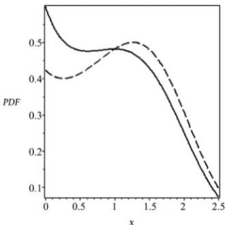
The two PDF’s are plotted in Figure 1, where the continuous line is the solu-tion according to Itô and the dashed line the solusolu-tion according to Stratonovich. The parameters take the values a=1,b=0.5,c=1,σ =1_{. In this case, the} differ-ences are not remarkable though there are. However, the variances are more dif-ferent: 0.439473 according to Itô, 0.519702 according to Stratonovich. The larger variance of Stratonovich’s solution is caused by the extra-term in Equation (19), which has opposite sign to the drift term.

3.2. Cubic System with Double Well Potential and Nonlinear

Parametric Excitation

We analyze the following nonlinear system

( )

3 ₂

( )

dX t =_aX t −bX t _dt+ c+σ X t Bd _{, (22)}

where a, b and c are real positive constants, and B(t) is a standard Brownian mo-tion. X(t) is allowed to assumed positive values only. This system has been ana-lyzed in many and many papers, but in most cases the excitation was additive. The restoring force derives from the potential function _ax2 ₂₋_bx4 ₄_{, which} has unstable maximum for x=0_{and two stable minima in} ± 2a b_.

According to Equations (13, 14) the first derivate moments is

( ) 3

1I

m =ax bx− _{. (23)}

( ) 3 2

1S ₄

m =ax bx− +σ . (24) in Itô’s and Stratonovich’s prescriptions, respectively. As in the previous case, the third term in Equation (24) equates the Wong-Zakai-Stratonovich corrective term, and the second derivate moment is _c₊_σ2_x_.

If the excitation is external, this system is known to have a bimodal PDF. With the parametric excitation of Equation (22) the PDF’s are

( )

_{( )}

(

)

3 2 2

2 2 4 2 6

3

2

4 8

2 2 2

exp 3

2 ln ,

I I

p x

c x

ac bc _c _x

σ σ σ σ σ

σ σ σ  = ⋅ _− + + − + _    + _− + _ + _    (25) ( )

_{( )}

(

)

3 2 2

2 2 4 2 6

3

2

4 8

2 2 2

exp 3 1

2 ln .

4

S S

p x

c x

ac bc _c _x

σ σ σ σ σ

σ σ σ  = ⋅ _− + + − + _    + _ − + _ + _    (26)

according to Itô and Stratonovich, respectively. With respect to Equations (20, 21) the terms with a change their signs. The two PDF’s are plotted in Figure 2

(Itô continuous line, Stratonovich dashed line): the parameters take the values

1, 0.5, 1, 1

(7)

[image:7.595.292.454.64.237.2] [image:7.595.290.455.279.444.2]

DOI: 10.4236/am.2019.1011063 882 Applied Mathematics Figure 1. Equilibrium PDF’s of the system (17): Itô’s solution

continuous line (___), Stratonovich solution dashed line (- - - -).

Figure 2. Equilibrium PDF’s of the system (22): Itô’s solution continuous line (___), Stratonovich solution dashed line (- - - -).

3.3. Cubic System with Double Well Potential and Strong

Nonlinear Parametric Excitation

The dynamical system of Section 3.2 now has a parametric excitation with a stronger nonlinearity:

( )

3 2 2

( )

dX t ₌aX t ₋bX t dt₊ c₊σ X t Bd

  , (27)

where a, b and c are real positive constants, and B(t) is a standard Brownian mo-tion. X(t) is allowed to vary on the whole real axis. The first derivate moments is

( ) 3

1I

m =ax bx− _{. (28)}

( ) 3 2

1S ₂

m =ax bx− +σ x. (29) in Itô’s and Stratonovich’s prescriptions, respectively. As in the previous case, the third term in Equation (29) equates the Wong-Zakai-Stratonovich corrective term, and the second derivate moment is _c₊_σ2 2_x _.

(8)

( )

_{( )}

2

(

2 2

)

2 2 exp 2 2 4 ln

I I

X C bx a bc

p x c x

c σ x σ σ σ σ

   

= ⋅ _− +_ + _ + _

+ _   _, (30)

( )

_{( )}

2

(

2 2

)

2 2 2 2 4

1

exp ln

2

S S

X C bx a bc

p x c x

c σ x σ σ σ σ

 _ _ 

= ⋅ _− +_ + + _ + _

+ _   _. (31)

according to Itô and Stratonovich, respectively.

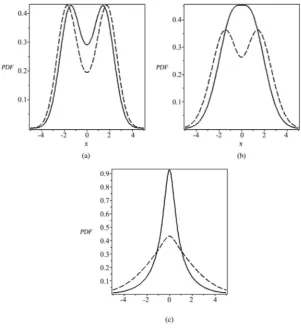
The PDF’s are plotted in Figure 3 for the following values of the parameters:

1, 0.25, 1

a= b= c= _{; the strength of the white noise σ varies. When the excitation} is external, this dynamical system has a bimodal PDF. The behaviour is different with the parametric excitation of Equation (27), as one can see in the plots: the look of the PDF depends on the value of σ. For values of σ lesser than one the PDF is bimodal in both approaches (Figure 3(a)). When σ =1₍_{Figure 3(b)}_),

[image:8.595.222.524.348.677.2]

the PDF is unimodal according to Itô, while it is bimodal according to Stratono-vich. Hence, according to Stratonovich the system has undergone a phase transi-tion. Raising σ to 3, both PDF’s are bimodal: thus, the phase transition in Itô’s interpretation is shifted to values of σ a bit larger. Because of the not simple expressions of the PDF’s, it is probably impossible to express the zeros of the first derivatives as functions of σ, but they can be found numerically.

Figure 3. Equilibrium PDF’s of the system (27) for σ=1 2 _(a),σ=1 (b), and

3

(9)

The differences in the PDF’s are notable especially in the last case in which they have a maximum only. However, the differences are really deeper as one can see in Table 1, where the variances are reported. In the Stratonovich’s ap-proach the variances are much larger than in Itô’s one. Moreover, they grow with σ, while according to Itô they diminish. It is concluded that in this case the two interpretations of the SDE’s lead to opposite behaviours of the system.

3.4. A Two-State System: Nonlinear Oscillator with Parametric

Excitation

Now we consider a nonlinear two-state oscillator with parametric excitations that has been already considered in literature according to the Itô’s interpreta-tion of the stochastic integral only [12] [13]:

( )

(

)

( )

2

( )

( ) ( )

( )

0 1 2 3

,

X t + f X X X t +

ω

X t = X t W t +X x W t W t + , (32) where f X X

(

,

)

_{is a deterministic function of the two states of the oscillator.}

W1, W2 and W3 are stationary independent Gaussian white noises with intensi-ties K jjj

(

=1,2,3

)

, and auto-correlations RW Wj j

( )

τ

=Kjj

δ τ

( )

. The FPK

equa-tions associated with Equation (32) are

(

)

{

(

)

}

(

)

1 2

1 2 1 2

2

0 1 1 2 2

1 2

2

2 2

11 1 22 2 33 2

2

,

, X X

X X X X

p

x p f x x x p

t x x

K x K x K

x ω ∂ ∂ ∂ = − _− _ ∂ ∂ ∂ ∂  

+ π _ + + _

∂

(33)

(

)

{

(

)

}

(

)

1 2

1 2 1 2

2

0 1 1 2 2 22 2

1 2

2

2 2

11 1 22 2 33 2

2

,

, X X

X X X X

p

x p f x x x K x p

t x x

K x K x K

x

ω

∂ _∂ _∂

= − _− + π _

∂ ∂ ∂

∂  

+ π _ + + _

∂

(34)

according to Itô and Stratonovich, respectively. Equation (34) differs from Equa-tion (33) because of the term πK x22 2 in the derivative with respect to x2.

In both cases the equilibrium PDF, if existent, has the form

(

)

(

)

1 2 1, 2 exp 1, 2

X X

p x x = ⋅C _−

φ

x x __{. (35)}

In Equation (35) φ

(

x x1, 2

)

is the probability potential that is solution to the first order ODE

(

) (

)

(

12 2 2 22

)

11 1 22 2 33

, d

d

f x x K

K x K x K

φ

λ

+ π =

[image:9.595.235.537.351.470.2]

π + + . (36)

Table 1. Variances for the system (27).

σ Itô Stratonovich

1 2 5.6363 7.2070

1 5.0122 7.6866

(10)

In Equation (36) the term in parenthesis in the numerator is absent in Itô’s interpretation; λ is a value of the mechanical energy Λ of the oscillator, that is

2 2 2

0 1 2

1 1

2ω X 2X

Λ = + _{. An admissible solution can be found if and only if the}

fol-lowing conditions hold [12] [13]

(

)

( )

2

1, 2 , 11 0 22

f x x = f

λ

K =

ω

K _{. (37)}

The second condition in Equation (37) imposes a rather restrictive relation-ship among the intensities of two excitations and a system parameter. Assuming that the conditions of Equation (37) are satisfied, the resulting PDF’s are

( )

₍

₎

( )

(

)

1 2 1 2

22 33

, exp d

2 I

X X I f

p x x C

K K

λ

λ λ

 

= ⋅ − _π ₊ 



∫

, (38)

( )

₍

₎

( )

(

)

1 2 1 2

22 33

, exp d

2 2 S S X X f C

p x x

K K K K λ _λ λ λ   = ⋅ _− _ π +

+ _

∫

_, (39)

according to Itô and Stratonovich, respectively.

For brevity’s sake, only the case f

( )

λ =aλ_{is presented. The integral in the}

exponentials is evaluated as

(

22 33

)

22 33

(

2222 33

)

ln 2 d

2 2 4

aK K K

a a

K K K K

λ

λ _λ λ

λ

⋅ +

= −

π + π π

∫

. (40)

In the numerical analyses the parameters take the values:

0 22

0.1, 2 , 0.1

a= ω = πK = _{in the first case, and}K₂₂=1.0_{in the second (K}₁₁

comes from the second of Equations (37)). The results of the first case are plot-ted in Figure 4 and Figure 5. Figure 4 shows the two-dimensional PDF given by Equation (38), say Itô’s interpretation and the two-dimensional PDF given by Equation (39) (Stratonovich’s). One can note that Itô’s PDF is rather flat around the maximum, while Stratonovich’s one is much more peaked. This fact is con-firmed by considering the sections X2 =0,p( )X XI₁ ₂=0 or p( )X XS₁ ₂=0 and

( )

2 1

1 0, X XI 0

X = p = or p( )X XS₂ ₁=0 that are shown in Figure 5. It is recalled that, strict-ly speaking, these functions are not PDF’s as they are not normalized: however, the normalization could be easily obtained numerically. A measure of the dis- persion is the mean square value, that is 2 ( )₁ ₂

1 X X 0d1

x p⋅ x

=

∫

or 2 ( )₂ ₁

2 X X 0d 2

x p⋅ x

=

∫

.

The dispersions of the section X1=0 are 0.030817 and 0.027244 according to

Itô and Stratonovich, respectively. The dispersions of the section X2 =0 are

7.644173 and 6.757889 according to Itô and Stratonovich, respectively. These values are not so different, and partly disavow the visible impression. However, on the whole the two PDF’s are different even if less than in other cases.

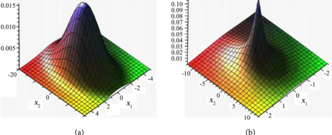
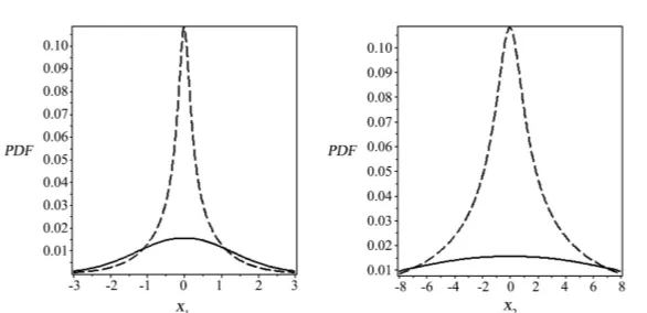
The results of the second case are in Figure 6, Figure 7: in Figure 6 there are the 3D plots of the joint PDF’s, while the sections X2=0,X1=0 are in Figure 7. As expected, the differences between the two interpretations of the stochastic differential Equation (32) are more marked in this case. In fact, the strengths

11, 22

K K of the parametric excitations are definitely larger: in this way, the term

22 2

K x

[image:10.595.231.535.215.291.2]

(11)

ab-DOI: 10.4236/am.2019.1011063 886 Applied Mathematics

sent in Itô’s interpretation). Even the mean square values are notably different: for the section X2 =0 they are 0.080475 and 0.055596 according to Itô and to

Stratonovich, respectively. For the section X1=0 the mean square values are

19.9617 and 13.7905, respectively. Performing the normalization, the variances

are 2 _1.6038

X

σ = _{and 0.8817 according to Itô and Stratonovich, respectively} with more notable differences.

[image:11.595.212.539.175.305.2]

(a) (b)

Figure 4. Two-dimensional PDF of the system (32) according to Itô, first case, Equation (38) (a), and according Stratonovich, Equation (39) (b).

[image:11.595.230.515.351.502.2]

(a) (b)

Figure 5. Sections X2=0 (a) and X1=0 (b) of the two-dimensional PDF’s of the

first case: Itô’s solution continuous line (___), Stratonovich solution dashed line (- - - -).

(a) (b)

Figure 6. Two-dimensional PDF of the system (32) second case K22=1.0, according to

[image:11.595.209.538.555.689.2]

(12)

[image:12.595.230.523.62.204.2]

DOI: 10.4236/am.2019.1011063 887 Applied Mathematics Figure 7. Sections X2=0 (a) and X1=0 (b) of the two-dimensional PDF’s of the

second case, K22=1.0: Itô’s solution continuous line (___), Stratonovich solution

dashed line (- - - ).

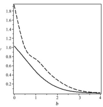
Another important aspect of the behaviour of a dynamic system is the mean upcrossing rate function νX

( )

b , that is the function that counts the times a stochastic process overpasses a given threshold b with positive velocity. For a second order system this function is given by Rice’s formula [35]:

( )

₀ _{1 2}

(

1 , 2

)

d 2

X b pX X x b x x

ν =

_∫

+∞ = . (41)

If one is interested in the outcrossings of the double barrier ±b_{and the PDF}

1 2

X X

p is symmetric, it is sufficient to double the result of Equation (41). In gen-eral, this is to be evaluated numerically.

In the case of high barriers, the upcrossings are rare events so that they can be considered independent and are assumed to constitute a homogeneous Poisson process. Thus, the cumulative distribution function of the first time T b

( )

at which the process X(t) crosses b firstly is given by

( )

_{1 e} X( )b

T

P T b_ _≤_τ_₌F _τ _{= −} −ν τ

  . (42)

From the usual laws of the probability it is obtained the important result

( ) (

]

( )

max 0, e X b

P_ X t

_τ

_≤b_₌ −ν τ

  . (43)

Thus, the knowledge of the mean upcrossing rate function yields an estimate of the largest value distribution of X(t): the estimate is as more precise as the upcrossings can be considered Poissonian.

As an example, Equation (41) has been numerically evaluated for the oscilla-tor of Equation (32) in the second case, that is with K22=1.0, considering

(13)

[image:13.595.292.460.66.240.2]

DOI: 10.4236/am.2019.1011063 888 Applied Mathematics Figure 8. Plot of the mean upcrossing rate function ν

( )

b against the barrier b for the oscillator of Equation (32) with K22=1.0: Itô’s

solu-tion continuous line (___), Stratonovich solusolu-tion dashed line (- - - -).

4. Conclusions

In this paper, the problem of the interpretation of the stochastic differential equ-ations is addressed from an applicative point of view. Theoretically, when eva-luating a stochastic integral with respect to a Brownian motion, there are infinite interpretations, and hence infinite values for the integral depending on the choice of the integration point. However, Itô’s interpretation and Stratonovich’s one are the most common so that attention is restricted to these two interpretations, even if the kinetic interpretation too is relevant. It has been underlined [36] that the interpretation of a stochastic differential equation has a deep deterministic root, residing in the integration rule that one adopts: Itô’s choice corresponds to the forward integration rule, while Stratonovich suggests the trapezoidal rule.

In order to highlight the differences in the responses that are obtained ac-cording the two interpretations of a stochastic integral, some stochastic dynamic systems with parametric excitation are analyzed, for all of which the FPK equa-tion has an analytical soluequa-tion in the final equilibrium regime. In the first three cases, the system is scalar. In the case of Section 3.1, the restoring force derives from a potential function with a minimum only: there are small differences be-tween the PDF’s of the two approaches, which however are present.

In the cases that are examined in Sections 3.2 and 3.3, the potential function has two stable minima and an unstable maximum in zero. When the excitation is merely external, the equilibrium PDF is always bimodal. It remains bimodal in both interpretations in the case of Section 3.2 that is characterized by a milder parametric excitation

(

_c₊_σ2_{X B}2_d

)

_{, but the PDF’s look very differently.}

In Section 3.3, the excitation is definitely more nonlinear

(

_c₊_σ2_{X B}2_d

)

_,

(14)

(Table 1).

The last case (Section 3.4) regards a second order oscillator, for which the problem of the mean upcrossing rate of a given level is also addressed. The res-ponses are not comparable, and the oscillator is safer according to Stratonovich than according to Itô.

The following conclusions can be drawn: 1) the two interpretations of a sto-chastic integral lead to marked differences in the statistical features of the re-sponse of a dynamic system. 2) Hence, caution is necessary in choosing an in-terpretation instead of the other. 3) Likely, Stratonovich’s inin-terpretation is pre-ferable as it has deeper physical bases, the respect of the law of the conservation of the energy and the agreement with the experiments. 4) However, one can equally use Itô’s stochastic differential calculus by modifying the original SDE with the addition of the Wong-Zakai-Stratonovich corrective term in the drift: in such a way Stratonovich’s solution is recovered.

In writer’s thought, the future work should follow two lines: 1) execution of experiments on dynamic systems with parametric excitation miming real cases; 2) theoretical studies regarding the effects of the different interpretations of a sto-chastic integrals on other aspects of the stosto-chastic dynamics such as stosto-chastic stability, first passage time problem, and white but not Gaussian excitations.

Conflicts of Interest

The author declares no conflicts of interest regarding the publication of this pa-per.

References

[1] Einstein, A. (1905) Über die von der molekularkinetischen Theorie der Wärme ge-forderte Bewegung von in ruhenden Flüssigkeiten suspendierten Teilchen. Annalen der Physik, 322, 549-560.https://doi.org/10.1002/andp.19053220806

[2] Langevin, P. (1908) Sur la théorie du mouvement Brownian. Comptes Rendus de l’Académie des Sciences, 146, 530.

[3] Fokker, A. (1914) Die Mittlere Energie Rotierender Elektrischen Dipole in Strah- lungsfeld. Annalen der Physik, 348, 810-820.

https://doi.org/10.1002/andp.19143480507

[4] Planck, M. (1917) Sitzungsber Preuss Akad. Wiss.Phys. Math. K1, 325.

[5] Kolmogorov, A.N. (1931) Über Die Analytischen Methoden in der Wahrschein- lichkeitsrechnung. Mathematische Annalen, 104, 415-458.

https://doi.org/10.1007/BF01457949

[6] Chandrasekhar, S. (1943) Stochastic Problems in Physics and Astronomy. Reviews of Modern Physics, 15, 1. https://doi.org/10.1103/RevModPhys.15.1

[7] Itô, K. (1951) On Stochastic Differential Equations. Nagoya Mathematical Journal, 3, 55-65.https://doi.org/10.1017/S0027763000012216

[8] Stratonovich, R.L. (1963) Topics in the Theory of Random Noise. Gordon Breach, New York.

[9] Hänggi, P. (1978) Stochastic Processes I. Asymptotic Behaviour and Symmetries.

(15)

[10] Klimontovich, Y.L. (1990) Itô, Stratonovich and Kinetic Forms of Stochastic Equa- tions. PhysicaA, 163, 515-532. https://doi.org/10.1016/0378-4371(90)90142-F

[11] Lin, Y.K. and Cai, G.-Q. (1995) Probabilistic Structural Dynamics: Advanced Theory and Applications. McGraw-Hill, New York.

[12] Cai, G.-Q. and Zhu, W.-Q. (2017) Elements of Stochastic Dynamics. World Scien- tific, Singapore.

[13] Gray, A.H. and Caughey, T.K. (1965) A Controversy in Problems Involving Random Parametric Excitation. Journal of Mathematics and Physics, 44, 288-296.

https://doi.org/10.1002/sapm1965441288

[14] Mortensen, R.E. (1969) Mathematical Problems of Modelling Stochastic Nonlinear Dynamic Systems.Journal of Statistical Physics, 1, 271-296.

https://doi.org/10.1007/BF01007481

[15] Ryter, D. (1978) Langevin Equations and Stochastic Integrals. Zeitschrift für Physik B Condensed Matter, 30, 219-222. https://doi.org/10.1007/BF01320988

[16] Srinivasan, S.K. (1978) Stochastic Integrals. SMArchives, 3, 325.

[17] West, B.J., Bulsara, A.R., Lindenberg, K., Seshadri, V. and Shuler, K.E. (1969) Sto- chastic Processes with Non-Additive Fluctuations: I. Itô and Stratonovich Calculus and the Effects of Correlations. PhysicaA, 97, 211-233.

https://doi.org/10.1016/0378-4371(79)90103-1

[18] van Kampen, N.G. (1981) Itô versus Stratonovich. Journal of Statistical Physics, 24, 175-187. https://doi.org/10.1007/BF01007642

[19] Smyth, J., Moss, F., McClintock, P.V.E. and Clarkson, D. (1983) Itô versus Strato- novich Revisited. Physics Letters A, 97, 95-98.

https://doi.org/10.1016/0375-9601(83)90520-0

[20] McClintock, P.V.E. and Moss, F. (1985) Further Experimental Evidence Pertaining to the Applicability of Itô and Stratonovich Stochastic Calculi to Real Physical Sys-tems. Physics Letters A, 107, 367-370.

https://doi.org/10.1016/0375-9601(85)90691-7

[21] To, C.W.S. (1988) On Dynamic Systems Disturbed by Random Parametric Excita-tion. Journal of Sound and Vibration, 123, 387-390.

https://doi.org/10.1016/S0022-460X(88)80121-4

[22] Di Paola, M. and Falsone, G. (1993) Itô and Stratonovich Integrals for Delta-Cor- related Processes. Probabilistic Engineering Mechanics, 8, 197-208.

https://doi.org/10.1016/0266-8920(93)90015-N

[23] Caddemi, S. and Di Paola, M. (1996) Ideal and Physical White Noise in Stochastic Analysis. International Journal of Non-Linear Mechanics, 31, 581.

https://doi.org/10.1016/0020-7462(96)00023-6

[24] Di Paola, M. and Pirrotta, A. (2004) Direct Derivation of Corrective Terms in SDE through Nonlinear Transformation on Fokker-Planck Equation. Nonlinear Dy-namics, 36, 349-360. https://doi.org/10.1023/B:NODY.0000045511.89550.57

[25] Braumann, C.A. (2007) Itô versus Stratonovich Calculus in Random Population Growth. Mathematical Biosciences, 206, 81-107.

https://doi.org/10.1016/j.mbs.2004.09.002

[26] Mannella, R. and McClintock, P.V.E. (2012) Itô versus Stratonovich: 30 Years Later.

Fluctuation and Noise Letters, 11, Article No. 1240010.

https://doi.org/10.1142/S021947751240010X

(16)

DOI: 10.4236/am.2019.1011063 891 Applied Mathematics https://doi.org/10.1088/1742-5468/2012/07/P07010

[28] Gonzales Arenas, Z. and Barci, D.G. (2012) Hidden Symmetries and Equilibrium Properties of Multiplicative White Noise Stochastic Processes. Journal of Statistical Mechanics: Theory and Experiment, 2012, P12005.

https://doi.org/10.1088/1742-5468/2012/12/P12005

[29] Hottovy, S., Volpe, G. and Wehr, J. (2012) Noise-Induced Drift in Stochastic Diffe-rential Equations with Arbitrary Friction and Diffusion in the Smoluchowski-Kra- mers Limit. Journal of Statistical Physics, 146, 762-773.

https://doi.org/10.1007/s10955-012-0418-9

[30] Aron, C., Barci, D.G., Cugliandolo, L.F., Gonzales Arenas, Z. and Lozano, G.S. (2016) Dynamical Symmetries of Markov Processes with Multiplicative White Noise.

Journal of Statistical Mechanics: Theory and Experiment, 2016, Article No. 053207.

https://doi.org/10.1088/1742-5468/2016/05/053207

[31] Sun, X., Duan, J. and Li, X. (2016) Stochastic Modelling of Nonlinear Oscillators under Combined Gaussian and Poisson White Noise: A Viewpoint Based on the Energy Conservation Law. Nonlinear Dynamics, 84, 1311.

https://doi.org/10.1007/s11071-015-2570-7

[32] Wong, E. and Zakai, M. (1965) On the Convergence of Ordinary Integrals to Sto-chastic Integrals. The Annals of Mathematical Statistics, 36, 1560-1564.

[33] Stratonovich, R.L. (1966) A New Representation for Stochastic Integrals and Equa-tions. SIAM Journal on Control, 4, 362-371. https://doi.org/10.1137/0304028

[34] Gardiner, C.W. (2004) Handbook of Stochastic Methods: For Physics, Chemistry and Natural Sciences. Springer, Berlin.

[35] Rice, S.O. (1944) Mathematical Analysis of Random Noise. The Bell System Tech-nical Journal, 23, 282-332. https://doi.org/10.1002/j.1538-7305.1944.tb00874.x

[36] Di Paola, M. (1993) Stochastic Differential Calculus. In: Casciati, F. Ed., Dynamic Motion: Chaotic and Stochastic Behaviour, Springer-Verlag, Vienna,29-92.