Solar Physics
DOI: 10.1007/•••••-•••-•••-••••-•
Null point distribution in global coronal potential
field extrapolations
S. J. Edwards1,2 · C. E. Parnell2 ·
c
Springer••••
AbstractMagnetic null points are points in space where the magnetic field is zero. Thus, they can be important sites for magnetic reconnection by virtue of the fact that they are weak points in the magnetic field and also because they are associated with topological structures, such as separators, which lie on the boundary between four topologically distinct flux domains and therefore are also locations where reconnection occurs. The number and distribution of nulls in a magnetic field acts as a measure of the complexity of the field.
In this paper, the numbers and distributions of null points in global potential field extrapolations from high-resolution synoptic magnetograms are examined. Extrapolations from MDI magnetograms are studied in depth and compared with those from high-resolution SOLIS and HMI.
The fall off in the density of null points with height is found to follow a power law with a slope that differs depending on whether the data is from solar maximum or solar minimum. The distribution of null points with latitude also varies with the cycle as null points form predominantly over quiet-Sun regions and avoid active-region fields. The exception to this rule are the null points that form high in the solar atmosphere and these null points tend to form over large areas of strong flux in active regions.
From case studies of the MDI, SOLIS and HMI data, it is found that the distribution of null points is very similar between data sets except, of course, there are far fewer nulls observed in the SOLIS data than the cases from MDI and HMI due to its lower resolution.
Keywords: Magnetic topology, magnetic fields, global corona, potential fields
1. Introduction
Magnetic null points are points in space where all three components of the magnetic field are equal to zero. They have long been recognized as impor-tant locations for reconnection (e.g., Dungey, 1953; Parker, 1957; Sweet, 1958;
1 Department of Mathematical Sciences, Durham University,
Durham, DH1 3LE. email:[email protected],2School of
Mathematics and Statistics, University of St Andrews, North Haugh, St Andrews, Fife, KY16 9SS. email:
Petschek, 1964). Reviews of more recent work on 2D reconnection can be found in Priest and Forbes (2000) and Biskamp (2000). Recently a body of work, which is still growing, has developed on the nature of reconnection at 3D nulls (e.g., Rickard and Titov, 1996; Bulanov et al., 2002; Pontin and Galsgaard, 2007; Priest and Pontin, 2009; Wyper and Jain, 2010; Al-Hachami and Pontin, 2010; Galsgaard and Pontin, 2011; Pontin, Priest, and Galsgaard, 2013; Wyper and Pontin, 2014). Additionally, null point reconnection has been identified as important in various observed solar flares (e.g., Aulanier et al., 2000; Fletcher
et al., 2001; Massonet al., 2009). The breakout model (Antiochos, DeVore, and Klimchuk, 1999) for coronal mass ejections (CMEs) is built upon the conjecture that reconnection at a high-altitude null point leads to an eruption causing a CME. Also, in the Earth’s magnetosphere null points have been identified from cluster data (e.g., Xiaoet al., 2006).
Furthermore, pairs of distant null points are frequently found to be connected by separators, which are also favourable reconnection sites (e.g.,Lau and Finn, 1990; Longcope, 2001, 2005; Longcopeet al., 2005; Hayneset al., 2007; Parnell, Haynes, and Galsgaard, 2008, 2010; Parnell, Maclean, and Haynes, 2010). Thus, establishing the number and spread of null points in the solar corona is an important step towards determining whether reconnection at null points and separators can play a key role in heating the solar atmosphere or whether they are crucial to events such as flares and CMEs.
Schrijver and Title (2002) investigated the distribution of null points in a region of quiet-Sun simulated by uniformly distributing point sources with fluxes taken from an exponential distribution over the base of their box. The potential magnetic field from these sources was then calculated throughout the box. They found that this gave an exponential fall off in the number of null points with height. However, since they took a simulated distribution of flux, their model is very much dependent on the parameters used in creating the flux distribution.
Close, Parnell, and Priest (2004) built on the work of Schrijver and Title (2002) by investigating the number of null points and separators above a patch of quiet-Sun field. First, they considered a magnetic field extrapolated from an exponential distribution of fluxes, similar to that used by Schrijver and Title (2002), and then they considered a sequence of observed magnetograms from MDI. The potential field above these magnetograms was determined by assuming that every magnetic fragment is a collection of point sources. Boundary effects were then eliminated by taking only the central region of the domain in which to determine the properties of the nulls and separators. An average of 1.051± 0.007 nulls were found per source, however, 96% of the nulls found were on the source plane.
The distribution of null points in a potential field extrapolated directly from a region of quiet-Sun observed byHinode/SOT was studied by R´egnier, Parnell, and Haynes (2008). Only one region of 102 Mm by 116 Mm was investigated in which 80 null points were found. All of these nulls lay above the base of the box, since the magnetic field on the base of the box is continuous. The number of null points was found to fall off linearly with height.
the distribution of null points in 562 high-resolution Michelson Doppler Imager (MDI) magnetograms of patches of quiet-Sun during the minima between Cycles 22 and 23 and between Cycles 23 and 24. Their approach could be applied provided the magnetic field extrapolations had the following properties: the mag-netic field was random with (i) homogeneous, Gaussian statistics and (ii) zero mean. Longcope and Parnell (2009) found that these conditions were met by their potential field extrapolations from many areas of quiet-Sun, but only at a height of about 1 Mm above the solar surface. Indeed, provided the field satisfies these conditions the expected null point distribution is a function only of the power spectral density (PSD) of the vertical photospheric field. Furthermore, the PSD analysis highlighted significant instrumental effects that meant during the many years of MDI data studied the numbers of nulls estimated “jumped”. Corrections were, therefore, made for both noise and this instrumental modulation function, before the null point distributions were estimated.
From their work, Longcope and Parnell (2009) calculated that the null column density, Nd(z), the number of nulls above a given heightz, is:
Nd(z) =
0.021
(z+ 1.5)2. (1)
A similar relationship was found for the number of nulls per unit volume,ρN(z),
as a function of height,z:
ρN(z) =
0.04
(z+ 1.5)3. (2)
These relationships were found to be independent of the magnetogram char-acteristics, such as spatial resolution. A result which was verified by Longcope, Parnell, and DeForest (2009), who used the same PSD method to analyse quiet-Sun magnetic fields observed by Hinode/NFI. When compared with the num-bers of nulls found directly in extrapolations from the magnetograms, the null distribution was found to have good agreement above 1.5 Mm.
All of the studies mentioned so far have considered the number of null points in local quiet-Sun regions. Cook, Mackay, and Nandy (2009) were the first to study the number of null points in a global field. They used a potential field source surface (PFSS) model (which considers a sum of spherical harmonics) to extrap-olate the coronal magnetic field from both smoothed synoptic magnetograms from the NSOVacuum telescope at Kitt Peak and from simulated photospheric magnetic fields based on these smoothed synoptic magnetograms. They found that the numbers of nulls varied in phase with the solar cycle and preferentially formed over active regions. However, in this study they neglected to include, in the simulated field, small-scale quiet-Sun fields, which, as discussed above, give rise to many null points. Also, all quiet-Sun fields were smoothed out of their synoptic magnetograms. Thus, the PFSS extrapolations, even though they had a maximum harmonic number oflmax= 63, only modelled the large-scale field.
However, the synoptic magnetograms they used were not subject to significant smoothing and so the global coronal fields could be modelled using a maximum harmonic number of lmax = 81. Thus, they were able to model much
smaller-scales than Cook, Mackay, and Nandy (2009). Platten et al. (2014) studied three solar cycles worth of data (496 synoptic maps corresponding to one each Carrington rotation). In contrast to Cook, Mackay, and Nandy (2009), they found that the most nulls occurred during solar minimum when extensive regions of mixed small-scale field are present on the solar surface.
Freed, Longcope, and McKenzie (2015) also directly identified null points in PFSS extrapolations of the global corona. However, their PFSS extrapolations have a low resolution, with anlmax= 30. The aim of their study was to see if, for
each null point found in the PFSS extrapolation, an observational signature of null points could be found inAtmospheric Imaging Assembly(AIA) images taken at the same time. Thus they were interested in null points that were situated fairly high in the solar atmosphere in regions that could be reasonably expected to be potential and also where the null points would be sufficiently isolated that the surrounding field might show an appropriate null-like structure. Not surprisingly, due to the low number of harmonics used, they found the number of null points to be in phase with the solar cycle, in agreement with the work of Cook, Mackay, and Nandy (2009).
In this paper, we extend the work of Plattenet al.(2014) and investigate null points found in global coronal potential fields extrapolated, using PFSS models with many harmonics, from high-resolution synoptic magnetograms taken by SOLIS, MDI and HMI. Here, we investigate the number and distribution of null points: both those nulls associated with quiet-Sun regions, as found by, e.g.,
Longcope and Parnell (2009) and also those associated with active regions, as studied by e.g. Cook, Mackay, and Nandy (2009) and Freed, Longcope, and McKenzie (2015).
2. Synoptic magnetic data and global potential field model
2.1. Magnetogram data
In this study, we focus mainly on global magnetic fields extrapolated from syn-optic magnetogram maps produced by the Michelson Doppler imager (MDI) aboardSolar and Heliospheric Observatory (SOHO). These maps are produced once every Carrington rotation (CR) and have a resolution of 3600 pixels in equal steps of longitude and 1080 pixels in equal steps of sine latitude. MDI was operational between May 1996 and November 2010. A total of 192 CR synoptic maps were produced during this time running from the minimum between Cycles 22-23 and the minimum between Cycles 23-24.
For comparison, we also include results from theHeliospheric Magnetic Im-ager (HMI) aboard the Solar Dynamics Observatory. These synoptic maps have a resolution of 3600 pixels in longitude and 1440 pixels in sine latitude. We analyse 49 such maps, one each CR, starting from CR2097 (20 May 2010).
Solar Observatory at Kitt-Peak. These maps have a resolution of 1800 pixels in longitude and 900 pixels in sine latitude. Again there is one map per CR starting from CR2007 (29th August 2003) giving us a total of 134 such maps.
2.2. Global potential field model
To extrapolate the global field from the synoptic maps a PFSS model (Schatten, Wilcox, and Ness, 1969; Altschuler and Newkirk, 1969) is used. This model ex-trapolates a potential field using spherical harmonics by making the assumption that, at a given radius (which we take to be 2.5R), the magnetic field becomes
purely radial.
In principal, an infinite number of harmonics should be summed to generate the potential field. However, the number of harmonics we use to extrapolate the potential field is dictated by the resolution of the input magnetic field maps and also by computational constraints. In order to minimise noise and to mitigate the effects of steep gradients between the discrete points in the data, we first smooth the synoptic magnetograms (using a Gaussian smoothing with a width of 0.5◦) before performing the PFSS extrapolation.
We sum the spherical harmonics up to a maximum harmonic numberlmax=
351 for the MDI and HMI data, which gives us a grid resolution of 1409 pixels in longitude, 705 in latitude and 206 exponentially spaced with radius. With the SOLIS data, we use a maximum harmonic number lmax = 301, which gives a
resolution of 1209 grid points in longitude, 605 in latitude and 177 exponentially spaced with radius. These particular values oflmax are chosen in order to
max-imise resolution (up to the computational limits of our machines), but at the same time minimise spherical ringing.
2.3. Finding the null points
We find the null points using the trilinear null finding method (Haynes and Parnell, 2007). This method assumes, for each 3D grid cell, the magnetic field to be linear along the edges of each grid cell, bilinear across the faces and trilinear in the 3D volume of the cell. The null points are found in three steps. First, the cells where there is no change of sign of each of the three magnetic field components are excluded. Second the intersection in a curve of the surfaces Bi = 0 and
Bj = 0 for two magnetic field components Bi and Bj is found within the cell
using trilinear interpolation. If the third magnetic field component changes sign along this line then the cell contains a null and we can use Newton’s method to find its sub-grid location. This method has been shown to be good for numerical fields. One limitation we have is that we cannot identify multiple nulls per cell and so we need to have a suitably fine grid structure.
3. Column density of null points
The column density of null points,Nd(z), as calculated by Longcope and Parnell
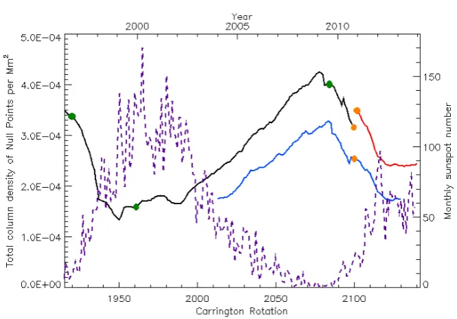
Figure 1. Total null column density per Mm2above the photosphere against time determined
from extrapolated global potential fields calculated using MDI (black line), high-res SOLIS (blue line) and HMI (red line) data. The sunspot number (purple dashed line) is plotted to indicate cycle phase. The times of the case studies examined in Section 6.2 are indicated by green dots and those considered in Section 6.1. are indicated by orange dots.
height. Figure 1 shows the total column density,Nd(0) (i.e.,the number of nulls
per unit area above z = 0, the solar surface) over time for all data sets with the sunspot number plotted for comparison. We can see that the total column density of null points is highest at solar minimum. This is to be expected, since there is more mixed polarity field at solar minimum so more null points form associated with small magnetic features. The blue line shows the total column density for the SOLIS data. This line is lower than the other two lines because the SOLIS data has a lower resolution, both in the input magnetogram and in the number of harmonics used for the extrapolation, than the MDI and HMI data and, as such, is unable to resolve as many small-scale magnetic features, so fewer null points are found.
From the MDI extrapolations (Figure 1, black line) we can see that the total column density varies from 4.5×10⁻⁴ nulls per Mm2 at solar minimum to 1.5
×10−4 nulls per Mm2 at solar maximum. This is, at all times, much lower than
the density of 6.8×10⁻³ nulls per Mm2 found by R´egnier, Parnell, and Haynes
where fewer nulls form than above purely quiet-Sun field, making the average density we determine less.
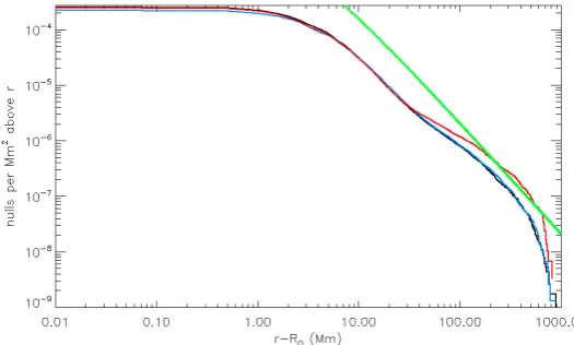
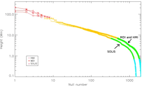
Figure 2. Variation of the null column density,Nd(r−R), against height above the solar surface,r−R, for MDI (black line), SOLIS high-resolution (blue line) and HMI (red line) extrapolations. The green line shows the fit found by Longcope and Parnell (2009).
To determine how the numbers of nulls fall off with height above the solar surface, we compare the column densities of null points,Nd(z), for the three data
sets (see Figure 2). All three data sets lie very close to one another. The SOLIS extrapolations (blue line) produce fewer nulls than the other two extrapolations below 1 Mm above the solar surface, since the resolution of the SOLIS data is lower. However, all the curves are essentially flat below a few Mm, because the number of nulls below this height are underestimated due to the use of just a finite number of harmonics in the PFSS model. Between 1 and 12 Mm above the solar surface, the three curves follow the same line as they fall off.
The HMI extrapolations produce more nulls for heights greater than 12 Mm above the solar surface than the MDI and SOLIS extrapolations. This is likely to be because the column densities are calculated by averaging over all the Carrington rotation frames observed by each instrument and, since HMI has been operational predominately during maximum, proportionally more nulls will have been produced at high heights associated with active regions.
The green line plotted in Figure 2 shows the relation found by Longcope and Parnell (2009) for comparative purposes. We see that the null column densities we find are closer to this relation at high heights than for lower heights, but in general they are always less than the column density predicted by Longcope and Parnell (2009). This behaviour can be explained.
(approximately unipolar). Longcope, Brown, and Priest (2003) showed that if either of these two characteristics were violated, then significantly fewer null points would be found. Thus, it is not a surprise that our null column density lies well below that estimated by Longcope and Parnell (2009).
The random nature of the magnetic field in radial cuts above the solar surface changes as the radial height increases. In particular, the small-scale features are lost and the length-scales become less varied with only large scales present. So, above 30 Mm, the field varies randomly in an more homogeneous manner than it does at the surface. This may be one possible reason why the null column densities all show a (slight) increase starting around 30 Mm. The increase in the HMI null column density is exaggerated since these observations are predomi-nantly taken during solar maximum. MDI and SOLIS both observe for a longer during solar minimum than solar maximum, but they still show an increase in null column density around 30 Mm.
Also, our PFSS extrapolations have an upper boundary (the source surface) at 2.5R, which lies 1.5R ≈103 Mm above the solar surface. This means the
numbers of nulls we find in our models drops off for large heights. Indeed, we find the numbers of nulls start to tailing off significantly around a 500-600 Mm. Longcope and Parnell (2009) have no upper boundary and so their prediction can be extended to arbitrary heights.
4. Null point distribution with height
We are interested in determining the distribution of null points with height. However, the distribution of null points will be different at solar maximum, when much of the solar surface is covered by active regions, than at solar minimum, when most of the solar surface is covered by quiet-Sun and there unipolar regions near the poles. With this in mind we take two subsets of the MDI data: Carrington rotations 1951 to 1989 to form a solar maximum data set and Carrington rotations 1909 to 1924 and 2051 to 2099 to form a solar minimum data set.
In order to test the nature of the distribution, we fit several standard dis-tributions to the data using the method of maximum likelihood estimation. We choose to only fit the distributions to null points that lie a few Mm above the photosphere, since, as can be seen from Figure 2, below this height the number of nulls tails off indicating that the resolution of our model is insufficient to reliably find all null points below this height.
The best fits to the data were found using a power-law-like probability dis-tribution function (pdf) of the form:
Nd(h;α) =
α−1 2h0
h+h 0
2h0 −α
Mm−2, (3)
where his the height above the photosphere, α, the power-law index, is a free parameter andh0 is the minimum height considered.
shallow so the best fit occurs whenh0= 2 andα= 2.51. At solar maximum the
value ofh0 that can be used is lower since there are less nulls low down during
this period and so fewer nulls at low heights are missed. At solar minimum, the resolution causes us to miss many low-altitude nulls so the best fit is when h0= 6 Mm. The form of the column density predicted by Longcope and Parnell
(2009) (Equation 1) was similar to this, except that it had a power-law index, α= 2 and anh0= 1.5 Mm. Our power-law indices are much greater in order to
[image:9.595.173.424.217.396.2]model the faster fall off in nulls that we find in our global fields.
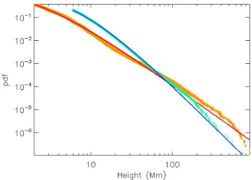
Figure 3. Probability distribution function of null points with height determined from the data for solar minimum (green diamonds) and solar maximum (orange stars) and model pdf from a power-law distribution withα= 3.52 andh0= 6 Mm(blue line) and (b)α= 2.51 and
h0= 2 Mm (red line).
Figure 3 shows the empirical and fitted pdfs of the distribution of null points with height for the solar maximum data (empirical pdf -orange stars and fit -red line) and also the solar minimum data (green diamonds empirical pdf and fit -blue line). These lines and points are only plotted for points aboveh0. The solar
minimum fitted curve falls off more steeply than the corresponding empirical pdf between 100 Mm and 300 Mm. The fitted curve for solar maximum shows a similar departure between 100 Mm and 600 Mm. Both curves cross the data again at high heights, where we see a fall off in the number of nulls owing to the boundary conditions.
5. Volume density of null points
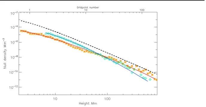
In Figure 4, we calculate, instead, the null volume density, ρN(z), with height.
Figure 4. Null volume density,ρN(h), plotted against height for PFSS extrapolations from MDI for solar minimum (green diamonds), solar maximum (orange stars) and the predicted null volume density from the fitted power law (Equation (7)), withα= 3.52 andh0= 6 Mm
(blue line) andα= 2.51 andh0= 2 Mm (red line). Black dashed line shows the fall off found
by Longcope and Parnell (2009) (Eq (2)).
The volume density of null points,ρN, can be estimated from the pdf,Nd(h;α)
fitted to the null column density (Equation (3)), as follows. First, we multiply Nd(h;α) by the number of nulls per frame, NF, and then integrate between
two heights,handh+δhand divide by the corresponding shell volume,V(h), between those two heights.
ρN(h;α) =
NF
V(h)
Z h+δh
h
α−1 2h0
t+h 0
2h0 −α
dt, (4)
where
V(h) = 4
3π (h+δh+R)
3−(h+R
)3, (5)
and R=696 Mm (solar radius).
Evaluating the integral in Equation (4) gives:
ρN(h;α) =−
3NF(2h0)α−1
4π
(h+δh+h
0)1−α−(h+h0)1−α
(h+δh+R)3−(h+R)3
. (6)
In the limit thatδh→0,
ρN(h;α) =−
NF(2h0)α−1(1−α)
4πR2
(h+h0)α(h+R)2
Mm−3. (7)
Unlike the prediction from Longcope and Parnell (2009), which suggested that the null volume falls as 1/(z+1.5)3, here we see that the rate of fall off varies with distance, h, from the solar surface. Equation (7) indicates that forhR the
The physical reason for this is that the volume of spherical shells increases with height so the null density falls off more rapidly, whereas in a Cartesian model, such as that used by Longcope and Parnell (2009), it remains constant. The curves plotted in Figure 4 are only weakly curved since there are no nulls at heights much greater than one solar radii.
From Figure 4, we can also see that, ifh≈h0thenρN(h) tend to a constant.
This means that for values ofhclose toh0 then slope of the null volume density
reduces/flattens.
In the solar maximum case (Figure 4, orange stars),α= 2.51<3, so, at low heights, the rate of fall off in the null volume density is slower than that predicted by Longcope and Parnell (2009). In contrast, the fall off at solar minimum is faster than that found by Longcope and Parnell (2009) since α= 3.52>3. As hincreases the rate of fall off steepens, so that, ath≈R, the fall off is either
1/h5.52 (minimum) or 1/h4.50 (maximum). Also, as already explained, the null volume density found in our model is, at all points, lower than that predicted by Longcope and Parnell (2009), since the magnetic field on the solar surface is not randomly distributed in a homogenous, Gaussian manner, but has a large variation in scales over the whole Sun.
6. Null butterfly diagrams
So far we have simply discussed the distribution of null points as a function of height above the solar surface. However, we are also interested in how null points are distributed across the solar disc. Sunspot and magnetic butterfly diagrams are often used to describe the latitudinal distribution of active regions on the solar surface, so we follow this approach here to investigate the distribution of nulls.
Both Cook, Mackay, and Nandy (2009) and Platten et al. (2014) created butterfly diagrams of the null points they found, but in both cases their data was of a much lower resolution than that used here and, hence, involved far fewer nulls. However, Plattenet al.(2014) have three solar cycles worth of data, including three solar minima: two with a strong dipolar field (i.e.,the minima between Cycles 21 and 22, and Cycles 22 and 23) and one with a weak dipolar field (minimum between Cycles 23 and 24). This allowed them to discover the interesting effect that null points occur at a higher heights during a weak polar minima than during strong polar minima. If the dipole field is strong then there is a strong magnetic connection between the solar poles. The magnetic field that links the poles holds in the weak, mixed-polarity, quiet-Sun field, which gives rise to coronal null points, hence these null point reside low in the solar atmosphere in a wide band around the equator. If the dipolar field is weak, then this field does not hold in the quiet-Sun field, i.e.,the magnetic influence of the mixed-polarity quiet-Sun field is relatively greater, therefore the volume of the corona in which null points can occur is greater.
lmax= 351, rather than lmax= 81. Thus many more null points can be found
[image:12.595.166.423.139.515.2]in the MDI extrapolations in comparison to the Kitt Peak extrapolations.
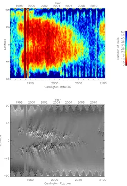
Figure 5. Null butterfly diagram for nulls found in PFSS extrapolations from MDI (top) and magnetic field butterfly diagram from MDI data (bottom).
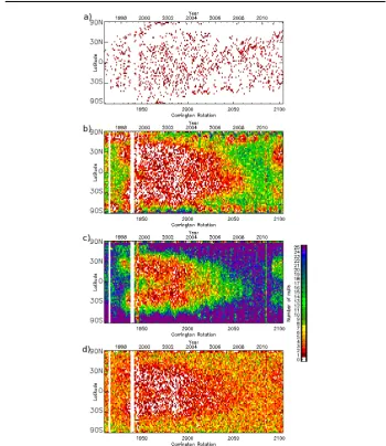
Figure 6. Null “butterfly diagram” for different height bands: (a)h >69.6 Mm, (b) 6.96 Mm
< h <69.6 Mm, (c) 0.696 Mm< h <6.96 Mm and (d)h <0.696 Mm. Colour indicates number of nulls present in a particular latitudinal band in each Carrington rotation, as indicated in the legend.
that in using low resolution PFSS extrapolations many null points below 69.6 Mm are missed.
As the number of harmonics in the PFSS model are increased, the null butterfly diagram tends towards that found in Figure 6b. This resembles the null butterfly diagram of Plattenet al.(2014) (Figure 20) for the PFSS model extrapolated from the Kitt Peak Vacuum Telescope and low-resolution SOLIS data using an lmax = 81. Here, we see that the nulls preferentially form away
from the activity bands, over mixed polarity quiet-Sun regions. This effect is accentuated for all heights below 69.6 Mm, but above 6.96 Mm (Figures 6c and 6d). Furthermore, between 6.96 Mm and 69.6 Mm the nulls occur less often over the streams of decaying active regions that head towards the poles at solar maximum than they do over proper quiet-Sun regions.
Since we hypothesise that the distribution of null points with height follows a power law, we would expect that the lowest height band (Figure 6d) would contain the most null points, but it does not. As we have already seen from Figure 2, our model does not have the resolution to find all the null points below 10 Mm and so Figures 6c and 6d are, in reality, missing many nulls.
7. Example cases
In addition to our long-term studies, we also compare the nulls found in indi-vidual frames taken either at the same time by different instruments or taken at different times by the same instrument. In particular, in Section 7.1, we investi-gate the nulls found in three different extrapolations of Carrington rotation 2100, which is in the crossover period of operation between MDI and HMI and is also observed by SOLIS. Following this, in Section 7.2, we make a detailed comparison of extrapolations from MDI taken at three different Carrington rotations: one from Cycle 23 maximum, one from the Cycle 22/23 minimum and one from the recent extended Cycle 23/24 minimum.
7.1. MDI vs. HMI vs. SOLIS - CR2100
To compare the results from data using three different instruments, we choose Carrington rotation 2100 which began on the 9th of August 2010 and was one of the first synoptic magnetograms produced by HMI, but one of the last produced by MDI. The Sun was near the beginning of the rise phase of Cycle 24. It had a number of active regions, but also had large areas of quiet-Sun. The polar fields at this time were fairly weak.
We would like to compare the distribution of null points to consider how robust this is to changes in the synoptic magnetogram due to instrumental (e.g.,spatial resolution, sensitivity and noise) or other effects (e.g.,synoptic map construction method, including the correction/estimation of the polar fields).
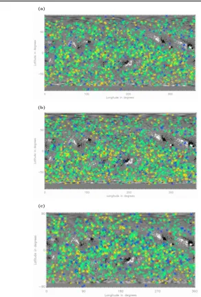
(a)
(b)
[image:15.595.129.422.88.520.2](c)
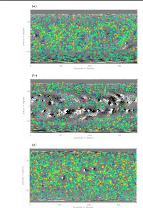
Figure 7. Positions of null points in the PFSS extrapolations for Carrington rotation 2100 from (a) HMI, (b) MDI and (c) SOLIS over-plotted on the corrseponding radial component of the magnetic field at the photosphere. Blue stars are nulls below 0.696 Mm, green stars are nulls between 0.696 Mm and 6.96 Mm, yellow stars are nulls between 6.96 Mm and 69.6 Mm and red stars are nulls above 69.6 Mm.
synoptic maps in Figure 7 and also Figure 8 which shows a comparison of the heights of all the nulls.
Figure 8. Heights of null points in the PFSS extrapolations for Carrington rotation 2100: HMI (diamonds), MDI (stars) and SOLIS (triangles). The colours represent the height bands:
h≤0.696 Mm - blue, 0.696 Mm< h≤6.96 Mm - green, 6.96 Mm< h≤69.6 Mm - yellow andh >69.6 Mm - red.
The high-altitude nulls that are not located at similar latitude and longitude in all three data sets are all very close to 69.6 Mm, so slight differences in the global dipolar field due to the lower order harmonics associated with the magnetic field at the poles could cause them to be classified in different height ranges and, hence, coloured differently. In fact, when we consider the locations of these high-altitude nulls (red stars in Figure 7) we see that all the nulls in the MDI extrapolation have corresponding null points in either the HMI or the SOLIS extrapolations or both. However, neither the HMI nor the SOLIS extrapolations show all the high-altitude nulls found in the MDI extrapolation. Furthermore, from Figure 8, it is clear that even if these high-altitude nulls are located at similar latitude and longitude they appear at heights that can differ by 50 Mm or more. This is likely to be due to the differing corrections applied to the polar fields in the creation of the synoptic maps. During the time of these observations there was a largeB-angle tilt leading to the South pole being poorly observed in all cases, thus, differences in polar field corrections are inevitable.
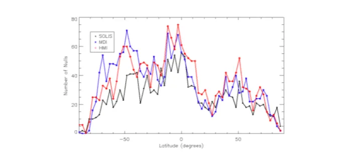
The latitudinal distribution of the null points (Figure 9) appears to basically be the same in all three models. There is a distinct asymmetry in the latitudinal distribution of nulls between the two hemispheres. This is a result of the asym-metry in the polar and active regions fields on the Sun at that time. Furthermore, the strength and size of the unipolar polar fields and the strongB-angle during this Carrington rotation will have a significant effect on the exactly nature of distributions, especially at higher latitudes. Additionally, the lower resolution of the SOLIS data means that this curve typically lies below the other two curves, as fewer nulls are observed overall by SOLIS.
Figure 9. Latitudinal distribution of null points in the PFSS extrapolations for CR2100 from HMI (black, crosses), MDI (blue stars), and HMI (red diamonds).
Table 1. Number and proportions of null points in different height ranges for the CR2100 extrapolations from MDI, HMI and SOLIS magnetograms.
MDI HMI SOLIS
Total number of nulls 2034 2113 1524
Resolution of input magnetogram 3600×1080 3600×1440 1800×900 Number of harmonics used (lmax) 351 351 301
No. nullsh >69.6 Mm 9 (0.4%) 6 (0.3%) 6 (0.4%) No. nulls 6.96< h <69.6 Mm 488 (24.0%) 473 (22.4%) 325 (21.3%) No. nulls 0.696< h <6.96 Mm 1325 (65.2%) 1379 (65.3%) 995 (65.3%) No. nulls 0< h <0.696 Mm 212 (10.4%) 255 (12.0%) 198 (13.0%)
than in the HMI or SOLIS extrapolations, however, in the HMI extrapolations this is balanced out by there being slightly more null points between 0.696 Mm and 6.96 Mm. The overall fall off in the height of the nulls is very similar, especially for the MDI and HMI extrapolations, which have the same maximum harmonic number and whose curves are indistinguishable where there is a high density of nulls,i.e., below 40 Mm. As we have already said, the height of null points can depend on the strength of the polar field, which is not well observed by any of the three instruments as they all observe along the Sun-Earth line. The different polar-field measurements and corrections used in the three data sets most probably causes the discrepancy in the numbers of nulls detected between 6.96 Mm and 69.6 Mm and also between 0.696 Mm and 6.96 Mm.
the fact that, although the numbers of SOLIS nulls start to fall off more quickly below 20 Mm than for the higher resolution models, the nature of the null height distribution is very similar in all three models. If this fall off in null numbers had occurred at a lower height then the proportions of the nulls in each height band would have appeared different.
7.2. CR1904 vs.CR1960vs.CR2083 - MDI
MDI was operational for two solar minima, but only one solar maximum so we take one frame from each minimum (CR1919 and CR2083) and one from the maximum in between (CR1960) to investigate the distribution of null points in detail.
In Figure 10, the positions of the null points found in each of these ex-trapolations, projected onto the photospheric synoptic magnetgrams for the corresponding Carrington rotation, are labelled as stars, with the star’s colour indicating the altitude of the null. From these maps it is clear that the mag-netogram data near the poles is not very good, so we are wary of drawing conclusions about the null points that are situated polewards of±70◦ latitude.
In the two solar minima examples (Figures 10a and 10c) the null points are distributed fairly evenly over the solar surface with most nulls low in the atmosphere. The only exception to this is above the small regions with relatively strong bipolar fields where there is a dearth of nulls. In Figure 10b, the solar maximum example, the spread of the nulls is found to be very different: far fewer null points form over the active regions than over the surrounding quiet-Sun regions, which lie polewards of ±40 degrees latitude. The few null points that do form above active regions are normally found at heights greater than 69.6 Mm above the photosphere (red stars in Figure 10b). This pattern, where the low altitude null points avoid the active-region bands, was shown clearly in the null butterfly diagrams (Figure 6) with nulls at heights less than 69.6 Mm preferentially situated away from the activity bands.
The latitudinal distribution of null points for these three cases is compared in Figure 11. The two solar minimum distributions are pretty similar and both peak roughly around the equator, however, the solar maximum distribution is as expected very different and highlights the dearth of nulls in the active region bands (equatorwards of ±40 degrees). Polewards of ±50 degrees latitude, the distribution of nulls is roughly similar to that found during the two solar minima, however, the strength and size of the polar fields and theB-angles during each Carrington rotation will have a significant effect on the nature of the distributions at these latitudes.
(a)
(b)
[image:19.595.131.427.88.517.2](c)
Figure 10. Positions of the nulls points found in the PFSS extrapolations of MDI synoptic magnetograms from (a) CR1919, (b) CR1960 and (c) CR2083 over-plotted on the radial component of the magnetic field at the photosphere. The stars show the projected position of the null points: blue stars are below 0.696 Mm, green stars are nulls between 0.696 Mm and 6.96 Mm, yellow stars are nulls between 6.96 Mm and 69.6 Mm and red stars are nulls above 69.6 Mm.
Figure 11. Latitudinal distribution of null points in the PFSS extrapolations from MDI for Carrington rotations: 1919 (black, crosses), 1960 (blue stars), and 2083 (red diamonds).
Figure 12. Heights of null points in the PFSS extrapolations from MDI for Carrington rotations: 1960 (cycle maximum, diamonds), 1919 (cycle minimum, stars) and 2083 (cycle minimum, triangles). The colours represent the height bands:h≤0.696 Mm - blue, 0.696 Mm
< h≤6.96 Mm - green, 6.96 Mm< h≤69.6 Mm - yellow andh >69.6 Mm - red.
Table 2. Number and proportions of null points in different height ranges for the extrapolations from MDI magnetograms from CR1919, CR1960 and CR2083.
Carrington Rotation 1919 1960 2083
Total number of nulls 1997 1017 2433
No. nullsh >69.6 Mm 3 (0.2%) 10 (1.0%) 6 (0.2%) No. nulls 6.96< h <69.6 Mm 387 (19.4%) 156 (15.3%) 635 (26.1%) No. nulls 0.696< h <6.96 Mm 1329 (66.5%) 706 (69.4%) 1566 (64.0%)
No. nulls 0< h <0.696 Mm 278 (13.9%) 145 (14.3%) 226 (9.3%)
8. Conclusions
In this paper, we have studied null points determined directly from global coronal magnetic fields created using PFSS extrapolations of MDI, HMI and SOLIS syn-optic magnetograms. In particular, we have investigated how the total numbers of nulls, the null column density and null volume density vary over the solar cycle and differ using data from the different instruments. Additionally, we have compared the locations and numbers of null points determined at the same Carrington rotation, but from three different synoptic maps (MDI, HMI and SOLIS), as well as undertaking a more detailed comparison of the locations of null points at different times during the solar cycle. From this work we can draw a number of interesting conclusions.
First though we discuss the limitations of using observed synoptic maps to extrapolate our global coronal field. The synoptic maps are constructed by taking successive latitudinal strip centred on the central meridian with a width of 13.5 deg longitude at the same time each day for 27 days. These are then placed side by side in order to create the synoptic map. Obviously this means that any active regions that emerge westwards of the central meridian are not observed until until that patch of Sun passes the central meridian again. Cook, Mackay, and Nandy (2009), who consider nulls in PFSS models extrapolated from simulated magnetograms that only included active regions, found that, by not counting these newly emerged active regions, they underestimated the numbers of null points. On the other hand, a newly emerged active region may actually reduce the amount of quiet-Sun field and since fewer nulls occur above active tas opposed to quiet-Sun regions, this effect may lead to an over estimation in the total number of nulls.
To begin with, the total number of null points, and, hence, the overall density of null points, varies out-of-phase with the solar cycle, but if we consider just high-altitude nulls the number varies in-phase with the solar cycle. This agrees with the results of Plattenet al.(2014) who found that nulls vary in phase with the solar cycle and explains the result of both Cook, Mackay, and Nandy (2009) and Freed, Longcope, and McKenzie (2015) who only studied high-altitude nulls, due to model limitations, and so found that nulls vary out of phase with the solar cycle.
The null points that are present low in the atmosphere preferentially form away from the locations of active regions and instead occur over quiet-Sun regions, whereas high-altitude null points tend to form over active regions and so are more prevalent at solar maximum. It is possible that small-scale reconnection events at the abundant low-lying null points, or at the multitude of separators that most likely connect many of these nulls, could contribute to coronal heating, but the models we have considered here do not have sufficient resolution to accurately determine the number of null points below 10 Mm.
A null column density falls off as (h+h0)−α for nulls above a heighth0. At
solar maximum, we get a good agreement with the data by lettingh0= 2 Mm
and anα= 2.51 and at solar minimum, we find the best fit by lettingh0= 6 Mm
and anα= 3.52. Both of these distributions have steeper gradients, especially at solar minimum, than that predicted by Longcope and Parnell (2009) (h0= 1.5
Mm and α = 2) for nulls above the quiet-Sun as observed by both MDI and NFI.
The null volume density was also investigated. In the predictions of Longcope and Parnell (2009), which uses a Cartesian model, the fall off in the null volume density is the same at all heights and goes as one over the height cubed. Our spherical model, however, has a different behaviour: nulls that are less than one solar radii above the solar surface have a null volume density that falls off at a rate proportional to (h+h0)−α (where, as above, α= 2.51 at solar maximum
and α = 3.52 at solar minimum), however, for nulls over a solar radii above the solar surface, the null volume density falls off much more rapidly at a rate proportional to (h+h0)−(2+α). This is simply due to the spherical nature of
the solar atmosphere rather than due to the fact that over 1.5 solar radii above the solar surface our model assumes that the magnetic field is purely radial. Thus, in our model the predicted fall off in null volume density is greater at solar minimum, than at solar maximum, but since at low heights there are more nulls at solar minimum, than at solar maximum, we find that these curves cross about 90 Mm above the solar surface.
The numbers of nulls found are dependent on the resolution of the model (through the amount/scale of the quiet-Sun fields considered), the instrument used to measure the photospheric magnetic field and the corrections made to the photospheric polar fields. This was shown in a comparison of null points found in PFSS models of the same Carrington rotation extrapolated from magnetograms from three different instruments. Although qualitatively the behaviour was the same in all the models, in terms of the locations of the nulls, the height and latitudinal distributions of the nulls, differences (often significant) were found when comparing individual null points at all heights. Even the highest nulls found did not necessarily have close relationship in terms of their height, latitude and longitude. This is believed to be due to the fact that even the very low spherical harmonics of the models can vary greatly due to the different corrections may to the polar fields.
In all cases, the numbers of nulls that we find in our models are less than those predicted by Longcope and Parnell (2009). This is not simply due to the lower resolution of the synoptic maps we use in comparison to the high resolution partial frame MDI data or NFI data considered by Longcope and Parnell (2009), but it is due mainly to the fact that the magnetogram data we consider is not random with homogenous, Gaussian statistics. Instead, it includes unipolar regions near the poles, active regions with large scale magnetic features and also regions of quiet-Sun with magnetic features with sizes varying over many scales. As explained by Longcope, Brown, and Priest (2003), magnetic fields that are not homogeneously random contain far few nulls than fields that are.
Platten et al. (2014) found just 40 to 120 null points from the PFSS ex-trapolations using low-resolution Kitt-Peak and SOLIS data, whereas here we have found between 1000 and 2000 using high resolution SOLIS data and even more (1000 to 2500) when either MDI or HMI data are used. This, as explained above, is due to the fact that the higher-resolution magnetograms allow (i) more randomness in the quiet-Sun fields to be detected producing more nulls, but also more spherical harmonics to be included in producing the coronal field extrapolations.
From the MDI data, we find a total column density of 4×10⁻⁴ nulls per Mm2, but the power-law fall off in null points means that a failure to resolve
small-scale features, which are associated with low-altitude null points, results in a large proportion of the null points being missed. In order to determine a more accurate column density of null points, global models from higher resolu-tion synoptic magnetograms using greater numbers of spherical harmonics are required to properly model the complexity of the magnetic fields below 10 Mm above the solar surface. However, it is clear from this work that the null points’ latitudinal and longitudinal distributions vary greatly over the solar cycle, as do their heights and total number.
References
Al-Hachami, A.K., Pontin, D.I.: 2010, Magnetic reconnection at 3D null points: effect of magnetic field asymmetry.Astron. Astrophys.512, A84.DOI.ADS.
Altschuler, M.D., Newkirk, G.: 1969, Magnetic Fields and the Structure of the Solar Corona. I: Methods of Calculating Coronal Fields.Solar Phys.9, 131.DOI.ADS.
Antiochos, S.K., DeVore, C.R., Klimchuk, J.A.: 1999, A Model for Solar Coronal Mass Ejections.Astrophys. J.510, 485.DOI.ADS.
Aulanier, G., DeLuca, E.E., Antiochos, S.K., McMullen, R.A., Golub, L.: 2000, The Topology and Evolution of the Bastille Day Flare.Astrophys. J.540, 1126.DOI.ADS.
Biskamp, D.: 2000,Magnetic Reconnection in Plasmas.ADS.
Bulanov, S.V., Echkina, E.Y., Inovenkov, I.N., Pegoraro, F.: 2002, Current sheet formation in three-dimensional magnetic configurations.Physics of Plasmas9, 3835.DOI.ADS. Close, R.M., Parnell, C.E., Priest, E.R.: 2004, Separators in 3D Quiet-Sun Magnetic Fields.
Solar Phys.225, 21.DOI.ADS.
Cook, G.R., Mackay, D.H., Nandy, D.: 2009, Solar Cycle Variations of Coronal Null Points: Implications for the Magnetic Breakout Model of Coronal Mass Ejections.Astrophys. J. 704, 1021.DOI.ADS.
Dungey, J.W.: 1953, Conditions for the occurrence of electrical discharges in astrophysical systems.Phil. Mag.44, 725.
Fletcher, L., L´opez Fuentes, M.C., Mandrini, C.H., Schmieder, B., D´emoulin, P., Mason, H.E., Young, P.R., Nitta, N.: 2001, A Relationship Between Transition Region Brightenings, Abundances, and Magnetic Topology.Solar Phys.203, 255.DOI.ADS.
Freed, M.S., Longcope, D.W., McKenzie, D.E.: 2015, Three-Year Global Survey of Coronal Null Points from Potential-Field-Source-Surface (PFSS) Modeling and Solar Dynamics Observatory (SDO) Observations.Solar Phys.290, 467.DOI.ADS.
Galsgaard, K., Pontin, D.I.: 2011, Steady state reconnection at a single 3D magnetic null point.
Astron. Astrophys.529, A20.DOI.ADS.
Haynes, A.L., Parnell, C.E.: 2007, A trilinear method for finding null points in a three-dimensional vector space.Physics of Plasmas14(8), 082107.DOI.ADS.
Haynes, A.L., Parnell, C.E., Galsgaard, K., Priest, E.R.: 2007, Magnetohydrodynamic evolu-tion of magnetic skeletons.Royal Society of London Proceedings Series A463, 1097.DOI.
ADS.
Lau, Y.-T., Finn, J.M.: 1990, Three-dimensional kinematic reconnection in the presence of field nulls and closed field lines.Astrophys. J.350, 672.DOI.ADS.
Longcope, D., Parnell, C., DeForest, C.: 2009, The Density of Coronal Null Points from Hinode and MDI. In: Lites, B., Cheung, M., Magara, T., Mariska, J., Reeves, K. (eds.)The Second Hinode Science Meeting: Beyond Discovery-Toward Understanding,Astronomical Society of the Pacific Conference Series415, 178.ADS.
Longcope, D.W.: 2001, Separator current sheets: Generic features in minimum-energy magnetic fields subject to flux constraints.Physics of Plasmas8, 5277.DOI.ADS.
Longcope, D.W.: 2005, Topological Methods for the Analysis of Solar Magnetic Fields.Living Reviews in Solar Physics2, 7.DOI.ADS.
Longcope, D.W., Parnell, C.E.: 2009, The Number of Magnetic Null Points in the Quiet Sun Corona.Solar Phys.254, 51.DOI.ADS.
Longcope, D.W., Brown, D.S., Priest, E.R.: 2003, On the distribution of magnetic null points above the solar photosphere.Physics of Plasmas10, 3321.DOI.ADS.
Longcope, D.W., McKenzie, D.E., Cirtain, J., Scott, J.: 2005, Observations of Separator Reconnection to an Emerging Active Region.Astrophys. J.630, 596.DOI.ADS.
Masson, S., Pariat, E., Aulanier, G., Schrijver, C.J.: 2009, The Nature of Flare Ribbons in Coronal Null-Point Topology.Astrophys. J.700, 559.DOI.ADS.
Parker, E.N.: 1957, Sweet’s Mechanism for Merging Magnetic Fields in Conducting Fluids.J. Geophys. Res.62, 509.DOI.ADS.
Parnell, C.E., Haynes, A.L., Galsgaard, K.: 2008, Recursive Reconnection and Magnetic Skeletons.Astrophys. J.675, 1656.DOI.ADS.
Parnell, C.E., Haynes, A.L., Galsgaard, K.: 2010, Structure of magnetic separators and separator reconnection.J. Geophys. Res. (Space Physics)115, 2102.DOI.ADS.
Parnell, C.E., Maclean, R.C., Haynes, A.L.: 2010, The Detection of Numerous Magnetic Separators in a Three-Dimensional Magnetohydrodynamic Model of Solar Emerging Flux.
Petschek, H.E.: 1964, Magnetic Field Annihilation.AAS-NASA Symposium on the Physics of Solar Flares (NASA Special Publication)50, 425.ADS.
Platten, S.J., Parnell, C.E., Haynes, A.L., Priest, E.R., Mackay, D.H.: 2014, The solar cycle variation of topological structures in the global solar corona.Astron. Astrophys.565, A44.
DOI.ADS.
Pontin, D.I., Galsgaard, K.: 2007, Current amplification and magnetic reconnection at a three-dimensional null point: Physical characteristics.Journal of Geophysical Research (Space Physics)112, 3103.DOI.ADS.
Pontin, D.I., Priest, E.R., Galsgaard, K.: 2013, On the Nature of Reconnection at a Solar Coronal Null Point above a Separatrix Dome.Astrophys. J.774, 154.DOI.ADS.
Priest, E., Forbes, T.: 2000,Magnetic Reconnection.ADS.
Priest, E.R., Pontin, D.I.: 2009, Three-dimensional null point reconnection regimes.Physics of Plasmas16(12), 122101.DOI.ADS.
R´egnier, S., Parnell, C.E., Haynes, A.L.: 2008, A new view of quiet-Sun topology from Hinode/SOT.Astron. Astrophys.484, L47.DOI.ADS.
Rickard, G.J., Titov, V.S.: 1996, Current Accumulation at a Three-dimensional Magnetic Null.
Astrophys. J.472, 840.DOI.ADS.
Schatten, K.H., Wilcox, J.M., Ness, N.F.: 1969, A model of interplanetary and coronal magnetic fields.Solar Phys.6, 442.DOI.ADS.
Schrijver, C.J., Title, A.M.: 2002, The topology of a mixed-polarity potential field, and inferences for the heating of the quiet solar corona.Solar Phys.207, 223.DOI.ADS. Sweet, P.A.: 1958, The Neutral Point Theory of Solar Flares. In: Lehnert, B. (ed.)
Electromag-netic Phenomena in Cosmical Physics,IAU Symposium 6, 123.ADS.
Wyper, P., Jain, R.: 2010, Torsional magnetic reconnection at three dimensional null points: A phenomenological study.Physics of Plasmas17(9), 092902.DOI.ADS.
Wyper, P.F., Pontin, D.I.: 2014, Non-linear tearing of 3D null point current sheets.Physics of Plasmas21(8), 082114.DOI.ADS.