Genetic algorithms for multiple choice problems

(1)

Choice Optimisation Problems

by

Uwe Aickelin

(Dipl Kfm, EMBSc)

School of Computer Science University of Nottingham

NG8 1BB UK [email protected]

Thesis submitted to the University of Wales

In candidature for the

Degree of Doctor of Philosophy

European Business Management School

University of Wales Swansea

(2)

This work has not previously been accepted in substance for any degree and is not

concurrently being submitted in candidature for any degree.

Signed ………. (Candidate)

Date ……….

Statement 1

This thesis is the result of my own investigations, except where otherwise stated. Other

sources are acknowledged by endnotes giving explicit reference. A bibliography is

appended.

Date ……….

Statement 2

I hereby give consent for my thesis, if accepted, to be available for photocopying and

for inter-library loan, and for the title and summary to be made available to outside

organisations.

(3)

Everybody has someone or something to thank for their success. Primarily I want to

use this opportunity to thank my supervisor Dr Kathryn Dowsland for her guidance and

support throughout my work. No doubt without the many of our discussions both this

thesis and my research would not have been possible. Additionally, I am very grateful

for the advice and support of Dr Bill Dowsland, the computer support staff and other

people of the European Business Management School. Furthermore, special thanks go

to Dr Jonathan Thompson for his early work on the nurse scheduling problem. I would

also like to thank my family who in their own ways always supported me. Finally,

thank you to Sonya for motivation, support and distraction at the appropriate times over

(4)

(5)

1 INTRODUCTION...1

1.1 THE NATURE OF THE PROBLEM...1

1.2 THE SOLUTION METHOD AND RESULTS...2

1.3 THE STRUCTURE OF THE THESIS...4

2 INTRODUCTION TO NURSE SCHEDULING...6

2.1 PROBLEM FORMULATION...6

2.2 INTRODUCTION TO NURSE SCHEDULING...14

2.3 CYCLIC NURSE SCHEDULING...15

2.4 LINEAR,INTEGER,CONSTRAINT AND GOAL PROGRAMMING...16

2.5 HEURISTIC SCHEDULING...19

2.6 META-HEURISTIC SCHEDULING...20

2.7 CONCLUSIONS...23

3 GENETIC ALGORITHMS FOR CONSTRAINED OPTIMISATION...25

3.1 GENETIC ALGORITHM INTRODUCTION...25

3.2 CONSTRAINED OPTIMISATION WITH GENETIC ALGORITHMS...28

3.3 IMPLEMENTING CONSTRAINTS INTO THE ENCODING...29

3.4 PENALTY FUNCTIONS...30

3.5 REPAIR...33

3.6 SPECIAL OPERATORS...36

3.7 DECODERS...37

3.8 MISCELLANEOUS METHODS...42

4 A DIRECT GENETIC ALGORITHM APPROACH FOR NURSE SCHEDULING ...47

4.1 ENCODING OF THE PROBLEM...47

4.2 DESCRIPTION OF EXPERIMENTS...52

(6)

4.4 DYNAMIC PENALTY WEIGHTS...68

5 AN ENHANCED DIRECT GENETIC ALGORITHM APPROACH FOR NURSE SCHEDULING ...75

5.1 EPISTASIS OR WHY HAS THE GENETIC ALGORITHM FAILED SO FAR? ...75

5.2 CO-OPERATIVE CO-EVOLUTION...78

5.3 SWAPS AND DELTA CODING...87

5.4 HILL-CLIMBER,REPAIR AND INCENTIVES...94

6 AN INDIRECT GENETIC ALGORITHM APPROACH FOR NURSE SCHEDULING ...103

6.1 WHAT IS AN ‘INDIRECT’APPROACH? ...103

6.2 PERMUTATION CROSSOVER AND MUTATION...105

6.3 THE DECODER FUNCTION...110

6.4 PARAMETER TESTING...119

6.5 DECODER ENHANCEMENTS...126

6.6 EXTENSIONS OF THE NURSE SCHEDULING PROBLEM...135

7 THE MALL LAYOUT AND TENANT SELECTION PROBLEM ...142

7.1 INTRODUCTION TO THE PROBLEM...142

7.2 SIMPLE DIRECT GENETIC ALGORITHM APPROACH...154

7.3 ENHANCED DIRECT GENETIC ALGORITHM APPROACH...164

7.4 INDIRECT GENETIC ALGORITHM APPROACH...173

7.5 FURTHER DECODER ENHANCEMENTS...179

7.6 NURSE SCHEDULING REVISITED...186

8 CONCLUSIONS AND FUTURE RESEARCH ...190

8.2 FUTURE RESEARCH...194

(7)

APPENDIX A GENETIC ALGORITHM TUTORIAL...209

APPENDIX B SUMMARY OF DIPLOM THESIS...222

APPENDIX C NURSE SCHEDULING DATA ...225

APPENDIX D ADDITIONAL NURSE SCHEDULING RESULTS...232

APPENDIX E MALL PROBLEM DATA ...242

(8)

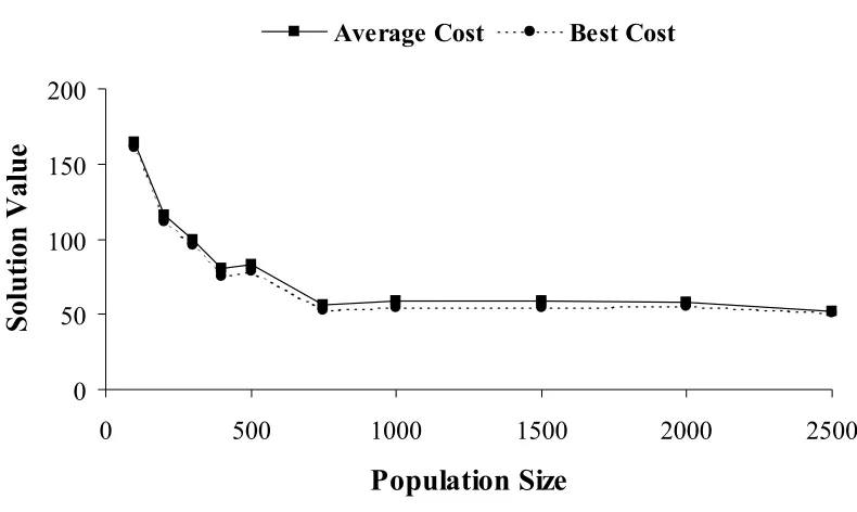
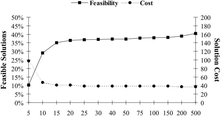
FIGURE 4-1:POPULATION SIZE VERSUS AVERAGE AND BEST SOLUTION COST. ...57

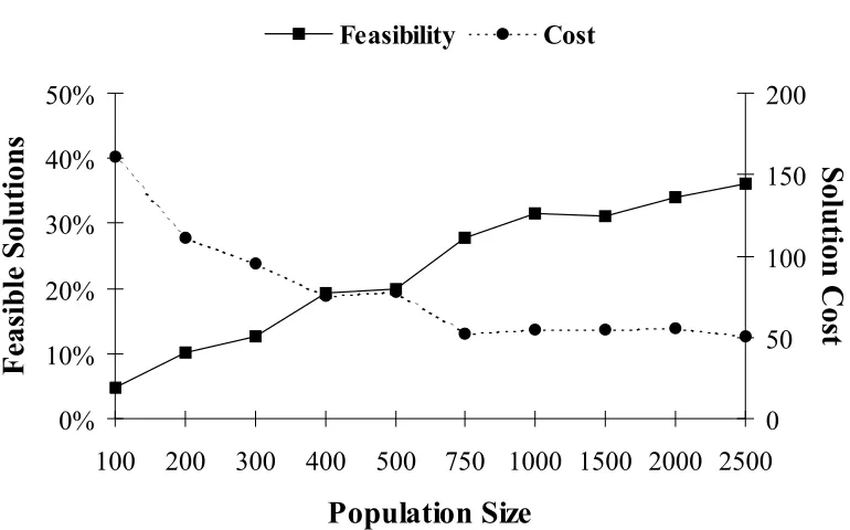
FIGURE 4-2:POPULATION SIZE VERSUS FEASIBILITY AND SOLUTION COST. ...58

FIGURE 4-3:POPULATION SIZE VERSUS SOLUTION TIME. ...58

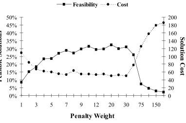
FIGURE 4-4:PENALTY WEIGHT VERSUS FEASIBILITY AND SOLUTION COST...59

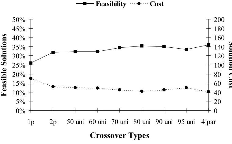
FIGURE 4-5:PERFORMANCE OF DIFFERENT TYPES OF CROSSOVER STRATEGIES...62

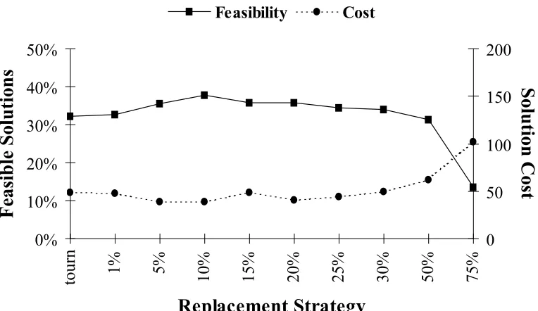
FIGURE 4-6:VARYING THE MUTATION RATE VERSUS FEASIBILITY AND SOLUTION COST. .63 FIGURE 4-7:COMPARISON OF DIFFERENT REPLACEMENT STRATEGIES. ...65

FIGURE 4-8:STOPPING CRITERIA VERSUS FEASIBILITY AND SOLUTION COST...66

FIGURE 4-9:STOPPING CRITERIA VERSUS SOLUTION TIME...67

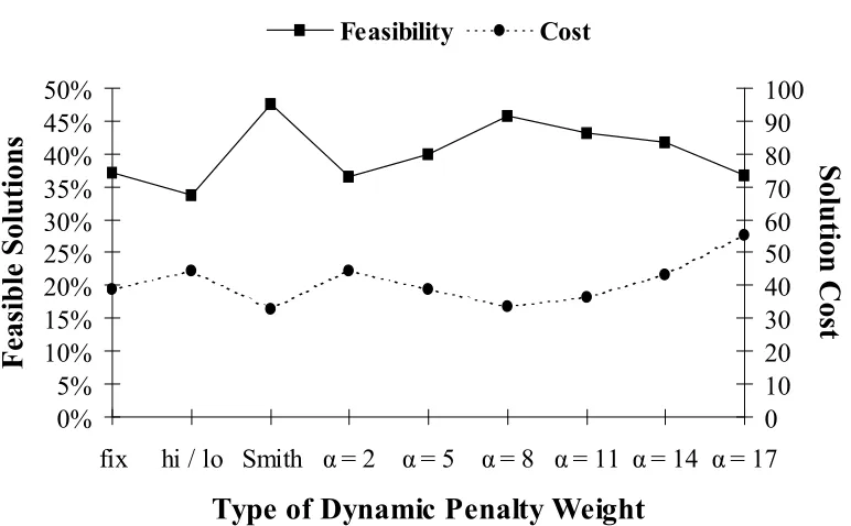
FIGURE 4-10:COMPARISON OF VARIOUS TYPES OF DYNAMIC PENALTY WEIGHT STRATEGIES...72

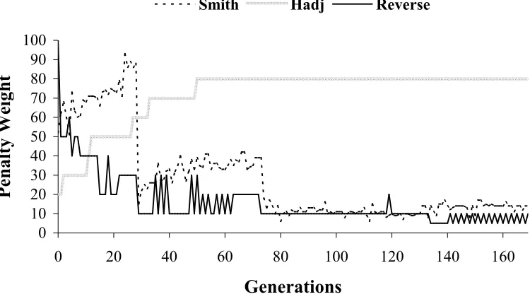
FIGURE 4-11:DEVELOPMENT OF DYNAMIC PENALTY WEIGHTS UNDER THREE STRATEGIES. ...73

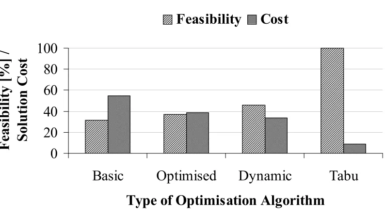
FIGURE 4-12:. COMPARISON OF SIMPLE DIRECT GENETIC ALGORITHMS WITH TABU SEARCH FOR NURSE SCHEDULING. ...74

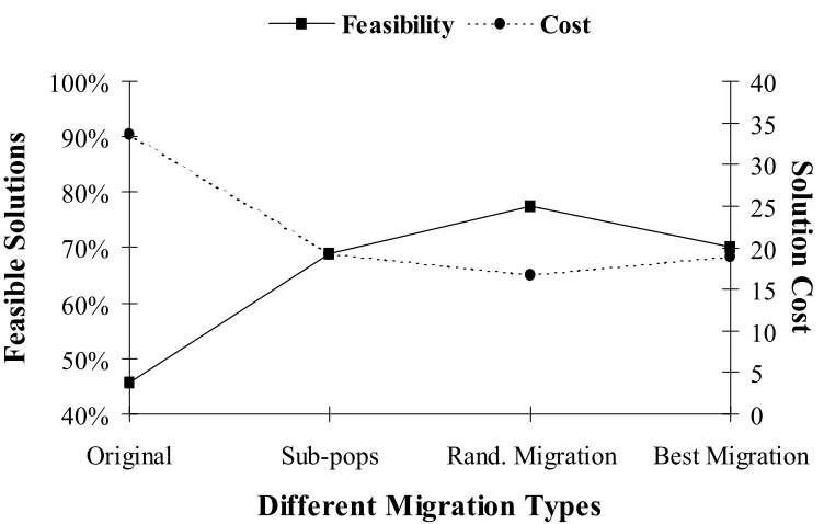
FIGURE 5-1:COMPARISON OF DIFFERENT MIGRATION TYPES WITH NO MIGRATION AND NO SUB-POPULATIONS...87

FIGURE 5-2:RESULTS FOR VARIOUS TYPES OF SWAPPING. ...90

FIGURE 5-3:COMPARISON OF SOLUTION QUALITY FOR VARIOUS DELTA CODING PROBABILITIES. ...93

FIGURE 5-4:DIFFERENT INCENTIVES (I), INCENTIVES AND REPAIR (R) AND DISINCENTIVES (D)...98

FIGURE 5-5:VARIOUS LOCAL HILLCLIMBING STRATEGIES. ...99

FIGURE 5-6: COMPARISON OF NURSE SCHEDULING RESULTS FOR VARIOUS DIRECT GENETIC ALGORITHM APPROACHES AND TABU SEARCH...102

FIGURE 6-1:EXAMPLE OF ORDER BASED CROSSOVER. ...106

FIGURE 6-2:EXAMPLE OF PARTIALLY MAPPED CROSSOVER (PMX). ...108

FIGURE 6-3:EXAMPLE OF ORDER BASED UNIFORM CROSSOVER. ...108

(9)

FIGURE 6-5:CROSSOVER OPERATORS AND OTHER VARIATIONS FOR THE OVERALL

CONTRIBUTION DECODER. ...123

FIGURE 6-6:WEIGHT RATIOS FOR THE OVERALL CONTRIBUTION DECODER...124

FIGURE 6-7:DIFFERENT SHIFT PATTERN ORDERINGS FOR THE OVERALL CONTRIBUTION DECODER...126

FIGURE 6-8:COMBINED DECODER WITH DIFFERENT PREFERENCE WEIGHTS. ...128

FIGURE 6-9:DIFFERENT TYPES OF CROSSOVER AND MUTATION. ...130

FIGURE 6-10:EXAMPLE OF CROSSOVER AND MUTATION BEFORE A BOUNDARY POINT. ..132

FIGURE 6-11:DIFFERENT WAYS OF USING BOUNDS. ...134

FIGURE 6-12:RESULTS OF THE EXTENDED NURSE SCHEDULING PROBLEM. ...138

FIGURE 6-13:. COMPARISON OF RESULTS FOR DIFFERENT DATA SETS BETWEEN THE DIRECT AND INDIRECT GENETIC ALGORITHM, TABU SEARCH AND XPRESSMP...140

FIGURE 6-14:COMPARISON OF GENETIC ALGORITHM APPROACHES WITH TABU SEARCH. ...141

FIGURE 7-1:FLOOR PLAN OF THE CRIBBS CAUSEWAY MALL NEAR BRISTOL...143

FIGURE 7-2:POPULATION SIZE VERSUS FEASIBILITY AND RENT. ...159

FIGURE 7-3:POPULATION SIZE VERSUS AVERAGE SOLUTION TIME. ...160

FIGURE 7-4:STOPPING CRITERIA VERSUS FEASIBILITY AND RENT. ...160

FIGURE 7-5:STOPPING CRITERIA VERSUS AVERAGE SOLUTION TIME...161

FIGURE 7-6:PENALTY WEIGHT VERSUS RENT AND FEASIBILITY. ...162

FIGURE 7-7:SINGLE BIT MUTATION PROBABILITY VERSUS FEASIBILITY AND RENT. ...163

FIGURE 7-8:CROSSOVER OPERATORS VERSUS RENT AND FEASIBILITY...164

FIGURE 7-9:COMPARISON OF VARIOUS TYPES OF DIRECT GENETIC ALGORITHMS. ...168

FIGURE 7-10:... VARIOUS INDIRECT GENETIC ALGORITHMS COMPARED WITH THE DIRECT APPROACH. ...179

FIGURE 7-11:FINAL AVERAGE WEIGHTS FOR TWO INITIALISATION RANGES AND DIFFERENT DATA SETS...182

FIGURE 7-12:DIFFERENT CROSSOVER STRATEGIES FOR THE INDIRECT GENETIC ALGORITHM...184

FIGURE 7-13:CROSSOVER RATES FOR ADAPTIVE CROSSOVER AND A ‘RELAXED’ FILE. ..185

(10)

FIGURE 7-15:CROSSOVER RATES FOR ADAPTIVE CROSSOVER AND A ‘TIGHT’ FILE...185

FIGURE 7-16:... VARIATIONS OF THE DECODER WEIGHTS AND CROSSOVER STRATEGIES FOR THE INDIRECT GENETIC ALGORITHM SOLVING THE NURSE SCHEDULING PROBLEM. 187 FIGURE 7-17:VARIOUS GENETIC ALGORITHMS FOR THE MALL PROBLEM...189

FIGURE I:ROULETTE WHEEL FOR FIVE INDIVIDUALS. ...213

FIGURE II:SCHEMATIC FOUR-POINT CROSSOVER. ...215

FIGURE III:EXAMPLE OF ONE-POINT CROSSOVER GOING WRONG FOR PERMUTATION ENCODED PROBLEMS. ...215

FIGURE IV:EXAMPLE OF C1 ORDER BASED CROSSOVER. ...216

FIGURE V:TYPICAL GENETIC ALGORITHM RUNS WITH VARIOUS STRATEGIES. ...232

FIGURE VI: COMPARISON OF AVERAGE SOLUTION COST FOR VARIOUS TYPES OF GENETIC ALGORITHMS AND A TYPICAL DATA SET. ...233

FIGURE VII: COMPARISON OF BEST FEASIBLE SOLUTION COST FOR VARIOUS TYPES OF GENETIC ALGORITHMS AND A TYPICAL DATA SET...234

FIGURE VIII:DETAILED RESULTS FOR BASIC GENETIC ALGORITHM. ...236

FIGURE IX: DETAILED RESULTS FOR A GENETIC ALGORITHM WITH DYNAMIC WEIGHTS AND OPTIMISED PARAMETERS...237

FIGURE X:DETAILED RESULTS FOR A CO-OPERATIVE CO-EVOLUTIONARY APPROACH. ..237

FIGURE XI: DETAILED RESULTS FOR A CO-OPERATIVE CO-EVOLUTIONARY APPROACH WITH REPAIR AND INCENTIVES. ...238

FIGURE XII:DETAILED RESULTS FOR AN INDIRECT GENETIC ALGORITHM WITH FIXED DECODER WEIGHTS...238

FIGURE XIII: .. DETAILED RESULTS FOR AN INDIRECT GENETIC ALGORITHM WITH DYNAMIC CROSSOVER RATES AND DECODER WEIGHTS. ...239

FIGURE XIV:QUADRATIC PENALTY WEIGHTS...240

FIGURE XV:MIGRATION OF FIVE BEST INDIVIDUALS OF EACH SUB-POPULATION...241

FIGURE XVI:RANDOM MIGRATION BETWEEN SUB-POPULATIONS...241

(11)

TABLE 4-1:INITIAL PARAMETER SETTINGS FOR THE DIRECT GENETIC ALGORITHM. ...54

TABLE 4-2:FINAL PARAMETER VALUES AND STRATEGIES FOR THE DIRECT GENETIC ALGORITHM...68

TABLE 5-1:EXAMPLES OF BALANCED, UNBALANCED AND UNDECIDED SOLUTIONS. ...95

TABLE 6-1: PARAMETERS AND STRATEGIES USED FOR THE INDIRECT GENETIC ALGORITHM AND NURSE SCHEDULING...120

TABLE 7-1:SPECIFICATIONS OF MALL PROBLEM DATA SETS. ...152

TABLE 7-2:INITIAL PARAMETERS AND STRATEGIES OF THE DIRECT GENETIC ALGORITHM. ...157

TABLE 7-3:PARAMETERS USED FOR THE INDIRECT GENETIC ALGORITHM. ...175

TABLE 7-4:THREE TYPES OF WEIGHT SETTINGS FOR THE MALL PROBLEM DECODER...178

TABLE I:EXAMPLE OF A WEEK’S DEMAND FOR NURSES. ...225

TABLE II:EXAMPLE OF NURSES’ GENERAL PREFERENCES AND QUALIFICATIONS. ...226

TABLE III:EXAMPLE OF NURSES’ WEEKLY PREFERENCES. ...227

TABLE IV:LIST OF ALL POSSIBLE SHIFT PATTERNS. ...230

TABLE V:EXAMPLES OF FINAL SHIFT PATTERN COST VALUES...231

TABLE VI:FULL GENETIC ALGORITHM, TABU SEARCH AND INTEGER PROGRAMMING RESULTS FOR ALL DATA SETS. ...235

TABLE VII:PROBLEM SIZE. ...242

TABLE VIII:LOCATION DISTRIBUTION...242

TABLE IX:GROUP MEMBERSHIP OF SHOP TYPES. ...242

TABLE X:LIMITS ON THE NUMBER OF SHOPS OF ONE SIZE...243

TABLE XI:EFFICIENCY FACTOR VERSUS SHOP COUNT...243

TABLE XII:ATTRACTIVENESS OF AREAS...243

TABLE XIII:LIMITS ON THE NUMBER OF SHOPS OF ONE TYPE. ...243

TABLE XIV:FIXED SHOP TYPE AND AREA RENT...244

TABLE XV:GROUP BONUS FACTORS...244

(12)

Multiple-choice problems come in many varieties: Choosing one’s lottery numbers,

deciding what to wear in the morning or assigning which shift pattern a nurse should

work. What all these problems have in common is that for each decision, be it a lottery

number, piece of clothing or a worker, there is only one object we can assign to it.

Hence, these are known as multiple-choice problems. Also, there are usually a number

of hard and soft constraints of different importance guiding our decisions. For instance,

it is only allowed to choose a particular lottery number once (hard constraint) or one

would like to wear clothes that match each other (soft constraint). This thesis uses

genetic algorithms to optimise multiple-choice problems, with the emphasis on

balancing those soft and hard constraints.

In this research, we will concentrate on two multiple-choice problems with covering

constraints. The research was motivated by the first problem to be tackled, which is to

find work schedules for nurses in a major UK hospital. The hospital operates 24 hours

per day using three shifts and nurses are graded into three bands. The required

schedules have to be calculated weekly and must consider various hard and soft

constraints. For instance, schedules must be perceived fair by staff and thus the

preferences of nurses, their past working history and other objectives have to be taken

into consideration. Furthermore, for each grade band and shift, strict covering

requirements are set which must be met.

This problem was chosen for a variety of reasons. It is a linear problem but difficult to

solve due to the multiple-choice component. Thus, although computationally

expensive, optimal solutions can be obtained for a comparison of results. Furthermore,

some insight into the problem structure existed from the tabu search approach reported

in Dowsland [55]. Additionally, the existence of a large number of real-life data sets

(13)

optimal solutions but to develop and compare new methods of handling constraints,

which can then be applied to more complex problems.

After developing suitable solution methods for this problem, we turn our attention to

mall layout and tenant selection. Although the problem and data in this case are

artificial, it is modelled closely after similar problems in real-life. This problem was

chosen as it is similar to yet more complex than the nurse scheduling problem. In

particular, the objective is non-linear. The aim is to place shops into locations of the

mall such that the overall revenue is maximised. This in turn maximises the rent

generated by the shops, the actual objective, as it is largely proportional to the revenue.

Constraints that have to be taken into account include upper and lower bounds on the

number of shops of one type and restrictions on the number of shops of a certain size

class. Soft constraints include some shops creating more revenue in certain areas of the

mall, synergy effects between similar shops and efficiency savings of larger shops.

1.2 The Solution Method and Results

The methods chosen to solve these multiple-choice problems are genetic algorithms.

They are inspired by evolution in nature and have the ‘survival of the fittest’ idea at

their heart. In contrast to other solution methods, they work with a population of

solutions in parallel and use stochastic crossover and mutation operators similar to those

found in nature. Recently, a lot of interest has been shown in using genetic algorithms

to solve real-life problems because of their flexibility and robustness. However,

canonical genetic algorithms are not function optimisers and in particular, there is no

explicit or generic way to include constraints. Thus, the purpose of this research is to

add to the knowledge in the area of constraint handling in a genetic algorithm

(14)

In a pilot study to this thesis (Aickelin [4]), it was shown that the nurse scheduling

example is both a difficult and interesting problem to apply genetic algorithms to.

Results for a very limited number of data sets were promising, although the main

stumbling block was as anticipated the constraints. It was concluded that once this was

overcome, the genetic algorithm would provide a robust and flexible solution method

for this problem. One of the first tasks of this research was to investigate if the results

found during the pilot study carry over for the much more extensive real-life data sets.

For further details of the pilot study, see the full summary, which is contained in

Appendix B.

Since the nurse scheduling problem is linear, optimal solutions for all data files are

known. This allows for a thorough comparison of the results of our various genetic

algorithm approaches. Additionally, Dowsland [55] solved the same problem with tabu

search. Both methods will be compared in terms of solution quality, robustness and

ease of including possible future expansions of the problem. Once successful genetic

algorithms are established, they are tested on the non-linear mall layout problem. This

allows for more general conclusions to be drawn about the suitability of our ideas for

1.3 The Structure of the Thesis

An introduction to genetic algorithms, their operators and the theory behind this type of

meta-heuristic can be found in Appendix A. A summary of the pilot study for the nurse

scheduling problem, assessing its difficulty and suitability to the proposed optimisation

approach, is given in Appendix B. The rest of this work is structured in the following

way.

Chapter 2 introduces the nurse scheduling problem in hand and a corresponding integer

program is set up. The remainder of the chapter looks at various solution methods to

nurse scheduling problems, with particular emphasis on linear programming and

meta-heuristic approaches. The chapter concludes that the approaches described in the

literature are not sufficient to solve the problem.

An overview of current genetic algorithm literature is given in chapter 3. The emphasis

of the chapter is on the treatment of constraints, as the pilot study found that the issue of

implementing constraints into a genetic algorithm framework is the most critical area of

the research. A detailed review of various methods, including penalty functions, repair,

decoders, special operators and others is given.

Chapter 4 details the encoding of our problem and presents the standard direct genetic

algorithm approach. After experimenting with various parameter and strategy settings,

the best values are retained. Then the first enhancement of the direct approach is

(16)

population. The chapter concludes with a summary of results and reasons for failure of

the methods used so far.

After discussing the issue of epistasis and its relevance to our research, chapter 5

presents co-operative and hierarchical sub-populations in an attempt to overcome the

problems encountered. Together with a special crossover operator and migration

between the sub-populations, this method is shown to be very effective at solving the

nurse scheduling problem. To improve upon the results, various further enhancements,

namely delta coding, swaps and a local hillclimber, are introduced next. The chapter

ends with a comparison of all direct genetic algorithm approaches used so far.

Chapter 6 is concerned with the indirect approach to the problem. After explaining the

idea of an indirect genetic algorithm, permutation based genetic operators, made

necessary by this type of genetic algorithm, are introduced. Then, some possible

decoders are detailed and shortened parameter tests are performed. Further

enhancements of the decoders and a new crossover operator are presented. Finally, the

original nurse scheduling problem is extended and it is shown that genetic algorithms

are flexible and robust enough to deal with this. The chapter concludes with a summary

and comparison of all nurse scheduling results.

To validate the results found so far, all previous methods are applied to the mall layout

problem in chapter 7. The superiority of the indirect over the direct approach is

confirmed and possible problems with the co-operative co-evolutionary approach are

discovered. Further enhancements of the indirect genetic algorithm are presented,

which after proving to be successful, are applied to the nurse scheduling problem as

well. A final comparison of results concludes the chapter.

The final chapter of this thesis summarises the findings of this project and makes

various recommendations as to the best way of solving multiple-choice problems with

genetic algorithms. This work is then put into the context of more general scheduling

(17)

2.1.1 General Introduction

This chapter gives details of the nurse scheduling problem tackled in this research and

presents an equivalent integer programming formulation. Following on from this, the

many ways in which similar problems have been solved by other researchers are

reviewed. A wide array of different methods has been proposed, all with their own

strengths and weaknesses. However, due to the nature of nurse scheduling problems,

most approaches described rely heavily on the particular problem structure, making

their use for our problem impossible.

Our task is to create weekly schedules for wards of up to 30 nurses at a major UK

hospital. These schedules have to satisfy working contracts and meet the demand for a

given number of nurses of different grades on each shift, while seen to be fair by the

staff concerned. The latter objective is achieved by meeting as many of the nurses’

requests as possible and considering historical information to ensure that unsatisfied

requests and unpopular shifts are evenly distributed. This will be further detailed in

section 2.1.3. For additional details, refer to Dowsland [55] and for example data to

Appendix C.

For scheduling purposes, the day at the hospital is partitioned into three shifts: Two day

shifts known as ‘earlies’ and ‘lates’, and a longer night shift. Note that until the final

scheduling stage, ‘earlies’ and ‘lates’ are merged into day shifts. Due to hospital policy,

a nurse would normally work either days or nights in a given week, and because of the

difference in shift length, a full week’s work would normally include more days than

nights. For example, a full time nurse works five days or four nights, whereas typical

part time contracts are for four days or three nights, three days or three nights and three

days or two nights. However, exceptions are possible and some nurses specifically

(18)

As described in Dowsland [55] the problem can be decomposed into the three

independent stages set out below. This thesis deals with the highly constrained second

step.

1. Ensuring via a knapsack model that enough nurses are on the ward to cover the

demand, otherwise introducing dummy and / or bank nurses to even out the cover.

2. Scheduling the days and nights on and off for a nurse.

3. Splitting the day shifts into early and late shifts using a network flow model.

2.1.2 The Three Solution Steps

In the following chapters, the nurse scheduling problem is often referred to as being

particularly ‘tight’. In order to understand this ‘tightness’ of the problem, one has to

know that all data is pre-processed by a knapsack routine to smooth out over- and

under-staffing. A knapsack is necessary due to the day / night shift imbalance, i.e.

nurses usually working more day shifts than night shifts. Hence, the knapsack

determines the maximum number of day shifts available subject to the night shifts being

covered. The consequence of this is that there is no slackness in most of the covering

constraints.

More precisely, the hospital requested that if any over-cover occurred it should be

spread out over day shifts only such that weekdays are covered first and weekends last.

To achieve this, additional dummy nurses are introduced who work as follows:

Weekend dummies can only work day patterns not including any weekdays. Weekday

dummies can only work day patterns not including any weekend days. They work as

many shifts as necessary to complement the over-cover to five days.

An example of the knapsack’s operation is as follows. Assume that there are 10 nurses

(19)

that the knapsack has found that 15 full time nurses are available to work days with the

remaining nurse required on nights. Since each full time nurse works five shifts, this

gives a total of 75 nurse shifts available on days. So overall, there is a surplus of five

nurse shifts. As the hospital requires the overstaffing to be spread over non-weekend

days first, the demand for Monday to Friday is raised by one shift each. This eliminates

the surplus and the knapsack routine is finished.

Now assume that one of the 15 nurses would only work four shifts in this week due to a

day off work. As before the demand for Monday to Friday will be increased by one

shift. In this case, this leads to an artificial ‘shortage’ of one shift. This is met with the

introduction of a weekday dummy nurse who works one day shift. Again the overcover

is smoothed out and the knapsack routine is finished. Situations with other

combinations of over- and under-staffing are met in a similar way. The following list

describes all possibilities grouped by the amount of over staffing, where a ‘unit’ refers

to one single nurse shift:

• More than seven units: The demand is raised by one for all seven days until the

over-staffing is by seven units or less.

• Seven units: The demand is raised by one for all seven days.

• Six units: The demand is increased by one for all seven days and additionally a

weekend dummy nurse is introduced.

• Five units: The demand is raised by one unit for weekdays only.

• Less than five units: The demand is raised by one unit for weekdays only and

additionally a weekday dummy nurse is introduced.

• If the knapsack determines that there are not enough nurses to cover the demand,

then as many bank nurses as necessary are introduced. Bank nurses can only work

one day shift each.

As ‘earlies’ and ‘lates’ are not yet merged at this stage, the second step of the problem

can be modelled as follows. Each possible shift pattern worked by a given nurse can be

represented as a zero-one vector with 14 elements, where the first seven elements

(20)

the vector denotes a scheduled day or night on and a 0 a day or night off. These vectors

will be referred to as shift patterns and examples can be found in appendix C.4.

Depending on the working hours of a nurse there are a limited number of shift patterns

available to her or him. For instance, a full time nurse working either 5 days or 4 nights

has a total of 21 (i.e.       5

7 _{) feasible day shift patterns and 35 (i.e.} _      4

7 _{) feasible night shift}

patterns. Typically, a nurse has around 40 possible shift patterns available to her / him.

Other data dimensions are between 20 and 30 nurses per ward, three grade-bands, nine

part time options and 411 different shift patterns.

The third step, the network flow algorithm, is of little interest to us. It splits the day

shifts into early and late shifts. The algorithm is always exact and takes little time to

find an optimal solution. Again, more details can be found in Dowsland [55].

2.1.3 Setting Up of the Nurse Shift Pattern Cost p

ij

Before setting up this problem, the cost pij of nurse i working shift pattern j has to be determined. This is done in the following way after close consultation with the hospital.

For each nurse, the number of day and night shifts she must work is given. Each of

these shift patterns is then assigned a ‘cost’ pij according to their suitability. For sample data of these costs and the factors that contribute to them, refer to Appendix C. More

precisely, the cost of a shift pattern is the sum of the following factors:

(1) Each shift pattern has been given a basic cost between one (no problems with

pattern) and four (very unattractive). This cost generally depends on whether the

pattern means that a nurse will have her days off together or separate. Note that

some patterns in which a nurse will work both days and nights are given a cost of

18. This cost is imposed if the shift pattern means that a nurse will work some night

(21)

(2) Nurses may prefer to work days or they may prefer to work nights. A nurse may be

classified as one of the following, depending on her or his contract and general

preferences:

• Days Only – in which case night shifts are not considered.

• Nights Only – in which case day shifts are not considered.

• Days Important – a cost of 12 is added to all night shifts.

• Nights Important – a cost of 12 is added to all day shifts.

• Days Preferred – a cost of 3 is added to all night shifts.

• Nights Preferred – a cost of 3 is added to all day shifts.

(3) A nurse may request not to work certain shifts and all shift patterns, which do not

satisfy these requests, are given a cost. Thus, if a shift pattern means that n requests are not satisfied, n costs are added. These requests are graded from one (relatively unimportant) to five (binding). Note that if a nurse requests not to work an early but

does not mind working a late, no cost is imposed as the nurse can be allocated a late

shift in the subsequent network flow phase. Likewise, for a nurse who requests not

to work a late but does not mind working an early. The costs added are:

• Grade 1 request – 3

(4) Nurses should not work more than seven days in a row. The cost added is equal to

the number of days above seven that they would have to work in a row.

(5) The shift pattern costs do not include continuity problems with previous schedules.

Thus, if the pattern a nurse worked last week finished 01, i.e. day off, day on; then

any shift pattern which begins with a day off is penalised by three. Likewise, a cost

of three is added if a nurse finished last week working 0 and starts this week

(22)

(6) Nights must be rotated: If a nurse worked nights last week, all night shift patterns

for this week have an additional cost of ten. If a nurse has worked nights the week

before, a cost of five is added.

(7) To rotate weekend work the following cost is added. If a nurse worked Saturday

and Sunday last week, a cost of one is added to each pattern that involves working

Saturday or Sunday this week.

(8) Before the problem is solved, one is deducted from the cost of each shift pattern for

each nurse. Thus, perfect shift patterns have a cost of zero. However, if the cost of

a shift pattern is above 89, it is set to 100. Costs for dummy and bank nurses are

always set to zero.

(9) Finally, the working history of a nurse is taken into account. If a nurse had a cost

for the shift pattern that she worked last week, then this is added to all non-zero cost

shift patterns (but not above 100).

2.1.4 Integer Programming Formulation

The problem can now be formulated as an integer linear program as follows.

Indices:

i = 1...n nurse index.

j = 1...m shift pattern index.

k = 1...14 day and night index (1...7 are days and 8...14 are nights).

(23)

Decision variables:    = else 0 pattern shift works nurse

1 i j

x_ij

Parameter:

n = number of nurses.

m = number of shift patterns.

p = number of grades.

   = else 0 night day / covers pattern shift

1 j k

a_jk    = else 0 higher or grade of is nurse

1 i s

q_is

pij = Penalty cost of nurse i working shift pattern j.

F(i) = Set of feasible shift patterns for nurse i.

Ni = Working shifts per week of nurse i if night shifts are worked.

Di = Working shifts per week of nurse i if day shifts are worked.

Bi = Working shifts per week of nurse i if both day and night shifts are worked.

Rks = Demand of nurses with grade s on day respectively night k.

Target function:

! min

1 ()

(24)

Subject to:

1. Every nurse works exactly one shift pattern:

i x

i F j

ij = ∀

∑

∈ 1 ) ( (1)

2. The shift pattern corresponds to the number of weekly working shifts of the nurse:

i shifts combined j B a or shifts night j N a or shifts day j D a i F i k jk i k jk i k jk ∀                           ∈ ∀ = ∈ ∀ = ∈ ∀ = =

∑

= = = 14 1 14 8 7 1 )

( (2)

3. The demand for nurses is fulfilled for every grade on every day and night:

s k R x a q _ks i F j n i ij jk is , ) ( 1 ∀ ≥

∑ ∑

∈ = (3)

Constraint sets (1) and (2) ensure that every nurse works exactly one shift pattern from

her feasible set, and constraint set (3) ensures that the demand for nurses is covered for

every grade on every day and night. Note that the definition of qis is such that higher graded nurses can substitute those at lower grades if necessary. This problem can be

regarded as a multiple-choice covering problem. The sets are given by the shift pattern

vectors and the objective is to minimise the cost of the sets needed to provide sufficient

cover for each shift at each grade. The multiple-choice aspect derives from constraint

set (1), which enforces the choice of exactly one pattern (or set) from the alternatives

available for each nurse. Although this problem looks similar to the generalised

assignment problem, it is different due to the additional shift pattern level, i.e. nurses

(25)

2.2 Introduction to Nurse Scheduling

There are many different ways of solving manpower scheduling and in particular nurse

scheduling problems. However, almost all solve a simplified version or are otherwise

very problem-specific, for example no grades are taken into account, all nurses are

assumed to be full time, or under- and over-staffing is allowed. During the course of

this research, it therefore became clear, that these methods could not be used to solve

our particular problem.

For the purpose of this chapter, nurse scheduling solution methods are classified into

four types following the recommendation of Bradley and Martin [27]: Exact cyclical,

heuristic cyclical, exact non-cyclical and heuristic non-cyclical. The problem in hand is

of a non-cyclical nature, because the hospital wants high flexibility to allow nurses their

requested days off and requests vary from week to week. Therefore, cyclical scheduling

approaches are only discussed briefly in section 2.3. The remainder of chapter 2 deals

with non-cyclical algorithms.

Exact non-cyclical solution methods, i.e. linear, integer and constraint programming, are

presented in section 2.4. The most commonly used algorithms are heuristic (section

2.5) and meta-heuristic (section 2.6). Although heuristic algorithms do not guarantee to

find the optimal solution, they tend to find very good solutions in a short time. The

term meta-heuristic refers to algorithms that contain a number of simpler heuristics.

This gives them the ability to be used for various problems with only slight

modifications. Examples of these methods are tabu search, simulated annealing and

genetic algorithms. In contrast, the methods of the heuristic section tend to be very

problem-specific and not suitable for other problems.

Many of the early approaches to manpower scheduling were of a manual nature. This

usually meant following a set of greedy rules when constructing a suitable roster. Due

to their limitations, they are not reported here in detail. The interested reader is referred

to Tien and Kamiyama [165] who give a good summary and comparison of many such

(26)

Bibliographies of more recent staff scheduling algorithms that concentrate on hospital

nurse scheduling are given by Hung [97], Sitompul and Randhawa [151] and Bradley

and Martin [27]. Additionally to the methods reviewed in this thesis, the authors

mention self-scheduling, that is the (manual) scheduling by the nurses themselves.

Self-scheduling is not further referred to in this thesis. The authors of the bibliographies

conclude that most methods surveyed are limited and that decision support systems or

the use of artificial intelligence might be possible future avenues for research.

2.3 Cyclic Nurse Scheduling

Cyclic nurse scheduling, as presented by Rosenbloom and Goertzen [141], is a common

way of solving the nurse scheduling problem. It first generates all possible basic work

patterns, usually on a weekly basis, by taking into account a variety of labour

constraints (work stretches, weekends off, no isolated days off or on etc). Furthermore,

only patterns that can be part of a larger schedule are allowed. For instance, if basic

patterns are for one week then for work-stretch constraints reasons, certain patterns

cannot be combined with others.

Once all feasible pattern pairs are determined, a linear programming optimisation

decides how often each pattern pair is used. Finally, the patterns are assigned to the

nurses who usually move onto a different pattern in every new planning horizon.

Hence, the name cyclic scheduling as nurses cycle through all patterns. For a practical

application of cyclic nurse scheduling, see Ahuja and Sheppard [3].

The nature of this approach is to regard all nurses as identical and hence no personal

preferences can be taken into account. At best, nurses can choose from the set of

optimal cyclic patterns. Our problem is not cyclic, because nurses’ preferences, which

will differ from week to week, must be taken into account. Thus, cyclic approaches

(27)

2.4 Linear, Integer, Constraint and Goal Programming

This section presents classical approaches that guarantee to find the optimal solution to

the non-cyclical problem. However, the drawback of this is the often prohibitively long

execution time. Thus, even though the problem formulation is still aimed at an optimal

solution, the actual execution is often of a heuristic nature, for example cyclic descent or

rounding of fractional variables rather than a full branch and bound approach.

One of the earliest examples of modelling the nurse scheduling problem as a

mathematical program can be found in Warner and Prawda [169]. The authors

formulate a linear program with the decision variables as the number of nurses of one

grade working a particular shift on a specific day. Should a solution become fractional,

a simple heuristic is used to correct it. To facilitate finding a solution, some substitution

between nurses of different grades is allowed. Furthermore, only an absolute lower

limit on the nurses required per shift is set. The target function is then to minimise any

staffing below the required level. No preferences or working constraints are taken into

account and the authors do not explain how to assign the shifts required in a solution to

the actual nurses.

Warner [170] presents an extension of the above. This time the problem is formulated

as an integer program, with the decision variables being the fortnightly shift patterns

worked by a nurse. As in our approach, each shift pattern is given a penalty cost.

However, Warner only bases this cost on work-stretch and isolated day on or off

preferences of the nurses. The number of possible shift patterns for each nurse is kept

small by having a fixed day and night rotation, alternate weekends off and further

restrictions. Limited under-covering of shifts is also allowed. The target function is to

minimise the sum of the costs of shift patterns for all nurses. The problem is solved via

a block pivoting heuristic. The solution found is then manually improved as far as

possible to form the final schedule.

Miller et al. [117] use the same problem formulation as Warner [170]. However, rather

(28)

setting constraints for maximum work-stretches and not allowing any isolated days on.

Nurses may request a particular day off which reduces the number of patterns further.

Moreover, they only consider full time nurses working ten days per fortnight and do not

distinguish between early, late and night shifts. The objective function is to minimise

under-staffing. The problem is solved with a cyclic descent algorithm.

A constraint programming approach to the nurse scheduling problem is given by Weil et

al. [171]. Constraint programming is similar to linear programming. However, rather

than a ‘blind’ branch-and-bound on the full domain of the decision variables, the

domains are dynamically reduced via the constraints in accordance with variables

already fixed. The problem formulation differs from ours, as nurses working a

particular shift on a specific day are the decision variables. The hard constraints are the

same as in our problem. However, Weil et al. considerably reduce complexity by only

scheduling full time nurses and not considering grades. Their objective is to minimise

the violation of soft constraints regarding isolated days on or off and work-stretches.

No individual preferences are considered. The authors are able to solve problems of

similar sizes to ours on a workstation within seconds. No solution quality is reported.

Cheng and Yeung [37] present a hybrid expert system combined with a linear zero-one

goal programming method to schedule full time nurses of one grade. The scheduling of

days on and off is done by the goal programming module. The goals are to satisfy

minimum staff levels, to minimise overtime, to grant requested days off, to limit

work-stretches to maximal six consecutive working days and to prevent off/on/off patterns.

For each goal, an aspiration level is set, for example the minimum required staff level

on a particular day. Each goal also has a priority level assigned to resolve conflicts.

The actual allocation to early, late and night shifts is done by the expert system

component, taking requests and required staff levels and other fairness measures into

account. An expert system consists of a set of rules of ‘if ... then ... else’ format. These

rules are gained by questioning experts, hence the name. The resulting hybrid system is

(29)

halving constraint violations. However, this approach would be unsuitable for us

because all goals have ‘soft’ aspiration levels, which is in conflict with our problem.

A similar goal programming approach is taken by Musa and Saxena [122]. In contrast

to Cheng and Yeung they include three grades and allow for various part time options.

However, they fail to include any preferences apart from the nurses choosing which one

out of two alternative weekends to be off work. The most similar goal programming

approach to our problem is given by Ozkarahan [124]. His problem is almost as

complex as ours, apart from only using two grades of nurses and not allowing any

substitution between the grades.

Arthur and Ravindran [7] present another two-phase goal programming heuristic to

solve their nurse scheduling problem. Only full time nurses are considered and the

three grades of nurses are scheduled independently. Since every other weekend is

strictly scheduled to be off, only five shift patterns are available to each nurse. The

goals are to meet the minimal staffing requirements and the individual preferences of

the nurses. Although the authors propose to extend their model to allow part time

nurses and to schedule all grades at the same time, it is not clear from the paper how

they will achieve this. Furthermore, there is no limit on the work-stretch length and the

model seems to rely on the use of an even number of nurses to function properly.

The nurse scheduling problem tackled in this thesis is also solved by Fuller [72] with

XPRESS MP, a commercial integer programming software package. When solved as

an integer program, as set up in section 2.1.4, optimisation times can be up to overnight.

Using different branching rules and a different formulation with additional variables and

constraints, computation time was reduced such that all files were solved within a

reasonable time frame. Her full results are reported and compared to our genetic

algorithm solutions in appendix D.2. These results show that in principle the problem is

solvable with branch and bound methods. However, sophisticated extensions and

(30)

2.5 Heuristic Scheduling

Gierl et al. [76] present a knowledge-based heuristic for scheduling physicians. Due to

the nature of their problem, no grades are taken into account. In addition, no personal

preferences are considered. Instead, an overall fairness measure is calculated. This is

based on the working history of each physician and aims at spreading out undesired

shifts and overtime. The algorithm then continuously cycles through all physicians,

assigning shifts to maximise the overall fairness.

A simple staff scheduling heuristic for full time nurses of one grade only is presented by

Anzai and Miura [6]. Cyclic descent and 2-opt heuristics are used to optimise the

schedule. Schedules of reasonable quality are found after some 90 seconds on an IBM

PC. However, the authors conclude that their model was too simplified which is to be

addressed in a yet unpublished future paper.

Kostreva and Jennings [104] solve the nurse scheduling problem in two phases. In the

first phase, groups of feasible schedules are computed. Each group fulfils the minimum

staffing requirements and each individual schedule all major working constraints. Then

in a second stage, the best possible aversion score is calculated for each group of

schedules. The aversion score is based on the preferences of each nurse and

corresponds to the pij values as described in section 2.1. The group of schedules with the lowest score is chosen. In contrast to our model, Kostreva and Jennings schedule all

grades independently from each other. Solution times are reported as approximately ten

minutes to generate one schedule on a Macintosh PC.

Blau and Sear [25] solve the problem using full time nurses of three grades, where

higher grades may substitute lower grades. In a first step they generate all possible shift

patterns over a two week period and evaluate them for all nurses based on their

preferences. The best 60 patterns for each nurse are kept and in a second step a cyclic

descent heuristic is used to find an optimal overall schedule taking both the nurses’

(31)

Decision support systems to solve the nurse scheduling problem are offered by

Randhawa and Sitompol [132] and by Smith et al. [153]. Both work in a similar way:

The usual constraints as well as nurses’ preferences are taken into account. The user is

asked to provide weights for various objectives. The algorithm then solves the problem

greedily. The focus of these decision support systems is on the interaction between the

user and the software, providing a what-if analysis for various sets of weights, rather

than optimal solutions.

2.6 Meta-Heuristic Scheduling

This section looks at examples of the use of meta-heuristics to solve the nurse

scheduling problem. The term meta-heuristic derives from the fact that these algorithms

contain many smaller heuristics inside them. This makes meta-heuristics very generic

in nature and they can often be used for various problems with only slight

modifications. The three meta-heuristics presented here are simulated annealing, tabu

search and genetic algorithms. For a concise summary and comparison of these three

approaches see Glover and Greenberg [77].

Simulated annealing is a neighbourhood search method where downhill moves are

always accepted and uphill moves are allowed under certain conditions to avoid being

trapped in local optima. The probability of an uphill move being accepted depends on

the change in the objective function value and on the temperature parameter. This

parameter controls the search and generally starts out high and then cools down

according to a cooling scheme. A higher temperature makes an uphill move more

likely.

Isken and Hancock [98] use simulated annealing to solve a variant of the nurse

scheduling problem. Their problem is more complex than the one tackled in this

(32)

shifts. On the other hand, complexity is reduced by the fact that they only schedule

nurses of one grade and that under- and over-staffing is penalised but allowed. The

problem is modelled as an integer program and then solved with a simulated annealing

heuristic. The authors found solutions within 25% of the optimal linear programming

solution in less than 15 minutes on a 386/25MHz personal computer.

Another popular meta-heuristic is tabu search. Tabu search is a neighbourhood search

method that usually accepts the best possible move. This can include uphill moves if no

downhill moves are available. To avoid cycling, a tabu list of the last few moves is

introduced. With every new move, the list is updated and moves currently on the list

must not be made. The main control parameter of tabu search is the length of the tabu

list.

Berrada et al. [21] formulate the nurse scheduling problem as a multi-objective

optimisation problem. The authors decompose the problem such that they schedule

early, late and night shifts separately and do not consider grades. The resulting problem

is modelled with covering constraints and nurses working their contracted number of

days as hard constraints and all other constraints (work-stretch, off/on/off patterns,

preferences) as soft constraints. The authors use both tabu search and standard

mathematical programming techniques to find pareto optimal solutions with regard to

the soft constraints. The results presented show that tabu search is capable of solving

the problem to the same quality as a commercial software packet (CPLEX), although

tabu search was much slower.

Burke et al. [32] also use tabu search on their nurse scheduling problem. However, as

their problem is of a very high complexity (planning horizon four weeks with up to 15

possible duties per day), they need to hybridise it with local search heuristics. The

results are of better quality than manual solutions and are usually found within minutes.

The same nurse scheduling problem as discussed in this thesis is also solved by

Dowsland [55]. Her tabu search algorithm uses a combination of different

(33)

solution and improving it in terms of preference cost. Furthermore, a succession of

problem-specific special neighbourhood moves is used to improve upon solutions

found. The final results match the quality of solutions produced by a human expert.

Her results and findings will be compared to ours throughout this thesis and full results

are reported in appendix D.2.

The final meta-heuristics presented in this section are genetic algorithms. As they are

our chosen method of solving the nurse scheduling problem they are explained in detail

in chapter 3 and in Appendix A. In a nutshell, genetic algorithms mimic the

evolutionary process and the idea of the survival of the fittest. Starting with a

population of randomly created solutions, better ones are more likely to be chosen for

recombination into new solutions. In addition to recombining solutions, new solutions

may be formed through mutating, i.e. randomly changing old solutions. Some of the

best solutions of each generation are kept whilst the others are replaced by the newly

formed solutions. The process is repeated until stopping criteria are met.

Easton and Mansour [56] use an enhanced genetic algorithm to solve an employee

staffing and scheduling problem. Their approach includes penalty functions to cope

with constraints (refer to sections 3.4 and 4.4), local hill climbing to improve solutions

(refer to sections 3.5 and 5.4), rank-based selection (refer to section 4.3.4) and

sub-populations (refer to section 5.2). The authors compare their results with those of

various other heuristics and manage to improve on the best results found so far on a set

of 36 test problems. No direct comparison of their tour scheduling problem to our

rostering problem is possible as their emphasis is on minimising the number of

employees needed to fulfil the schedule and does not take personal preferences into

account.

Tanomaru [164] uses a genetic algorithm based heuristic for a staff scheduling problem

of similar complexity to ours. He also has a weekly planning horizon and employees of

distinct grades. However, rather than using a three shifts approach (early, late and

night), employees can start at any time on the hour. Thus, solutions are represented by a

(34)

In contrast to our problem, the number of employees is not fixed and overtime is

allowed. Hence, the author’s objective is to minimise total wage cost. His algorithm

also makes use of penalty functions to cope with constraints such as total workforce

requirements and maximum individual working shifts.

To reduce the number of infeasible solutions, crossover is only allowed such that

‘whole employees’ are exchanged. The major optimisation work is then done by a set

of nine different heuristic operators. They act as a very sophisticated mutation operator

on a single employee basis. Solutions for moderate sized problems obtained after ten

minutes on a workstation were of similar quality as those of a human expert. Again,

Tanomaru shows the capabilities of genetic algorithms to solve highly complex

problems. However, he fails to report to what extent the nine heuristics used are

responsible for his results, which makes a comparison to our findings difficult. He also

concludes that for real-life problems, his heuristic mutation operators might be too time

consuming and suggests a parallel implementation for speed-up.

2.7 Conclusions

As the literature review shows, a lot of interest has been paid to the area of nurse

scheduling. This indicates that the problem is both interesting and difficult to solve.

However, due to the nature of nurse scheduling problems, problem-specific knowledge

was required in most cases to achieve good results. This makes it difficult to impossible

to include any specific ideas into our model. For instance, cyclic models cannot be used

due the importance of the nurses’ preferences in our example. Nevertheless, it has been

shown that heuristic approaches and in particular genetic algorithms have been

successful at solving similar problems.

Two methods have been suggested to solve the same nurse scheduling problem as is

(35)

Fuller [72]. As has been shown in section 2.1.4, the nurse scheduling problem shares

some similarities with set covering and generalised assignment problems. Fuller takes

advantage of this and uses an advanced integer programming approach to solve our

problem. However, this relies on having access to a sophisticated software package and

can involve up to overnight computer runs. Nevertheless, the results found by Fuller

allow for a thorough comparison and assessment of our results.

Results found by Dowsland are also of excellent quality. However, her algorithm is

domain dependent due to the special moves employed. For instance, some moves take

advantage of the fact that if one shift pattern containing a particular day is unfavourable

so are all others containing this day. This reduces the robustness of her algorithm. In

section 6.6, it is shown that this leads to poorer solution quality for more random data.

This leaves room for improvement for the genetic algorithm to capitalise on. As

mentioned earlier, genetic algorithms are well known to be very robust for a variety of

problems and data. In particular, as the section on meta-heuristic approaches has

shown, genetic algorithms have been successful in solving similar manpower problems.

Moreover, an earlier pilot study by Aickelin [4] had shown that using genetic

algorithms is a challenging but promising approach for this particular problem. The

pilot study concluded that the focus point of any future research into solving the nurse

scheduling problem with genetic algorithms has to be the handling of the problem’s

constraints. The next chapter will outline current research into genetic algorithms and

(36)

3.1 Genetic Algorithm Introduction

Due to the increasing popularity of genetic algorithms, a vast amount of research has

been published in this area. Thus, no literature review could possibly contain all the

information available. Moreover, as mentioned earlier, it was established in the pilot

study that the focus of future research into solving nurse scheduling problems with

genetic algorithms has to be the successful treatment of constraints. Therefore, this

literature review will concentrate on this area. Throughout this chapter examples of

related problems, such as scheduling, set covering and generalised assignment

problems, are used wherever possible.

However, beforehand this section will introduce the current state of research into

genetic algorithms for optimisation purposes. Note that there will not be an extensive

explanation of their actual workings. A more precise genetic algorithm tutorial based

on Davis [48] and Whitley [174] can be found in Appendix A. Good textbooks on the

topic are Goldberg [81] for earlier work up to 1989 and Michalewicz [115], Mitchell

[119] and Bäck [9] for more recent research. After a quick summary of the main

features of genetic algorithms, this section will go on to discuss recent research about

the merits of using them for function optimisation. The remainder of this chapter will

review the relationship between genetic algorithms and constraints.

Genetic algorithms are generally attributed to John Holland [96] and his students in the

1970s, although evolutionary computation dates back further (refer to Fogel [68] for an

extensive review of early approaches). Genetic algorithms are stochastic

meta-heuristics that mimic some features of natural evolution. Canonical genetic algorithms

were not intended for function optimisation, as discussed by De Jong [51]. However,

slightly modified versions proved very successful. For an introduction to genetic

(37)

implementations can be found in Bäck [8], Chaiyaratana and Zalzala [35], Hedberg [91]

and Ross and Corne [142].

To optimise a function, possible solutions are first encoded into chromosome-like

strings, in order that the genetic operators can be applied to them. Genetic algorithms

start with a population of usually randomly generated solutions. The two main genetic

operators are crossover and mutation, both loosely based on their natural counterparts.

The crossover operator takes (usually) two solutions, the so-called parents, and

recombines them to form one or more new solutions, the so-called children. Parents are

chosen from amongst all the solutions of the current population. However, the selection

is stochastically biased towards solutions with better objective function values. These

are also known as solutions with a higher fitness in evolutionary terms. Therefore,

genetic algorithms follow Darwin’s theory of ‘survival of the fittest’.

Mutation takes one solution and modifies it slightly to form a new solution. After

performing a certain number of crossovers and mutations, some of the solutions in the

old population are replaced by new solutions and this concludes one generation of the

algorithm. These generations are then repeated until a stopping criterion is met. Many

additional features are usually necessary in order to optimise real-life problems: Elitism,

i.e. the automatic survival of the x% best solutions, is used to preserve the best solution throughout generations. Additionally, some form of fitness scaling or ranking is often

necessary for a robust performance. However, one major problem remains. How does

one optimise constrained functions with genetic algorithms, which were originally

intended for unconstrained problems? This issue will be discussed in more detail in

section 3.2.

The inner workings of a genetic algorithm are often described in terms of the building

block hypothesis. The hypothesis says that short low-order solution sub-strings, also

known as schema, with higher than average fitness will be reproduced exponentially

and spread throughout the population. This is because of the Darwinian selection of

parents. The crossover operator then combines such schema or building blocks to form

(38)

Two articles discussing the merits of genetic algorithms for operational researchers are

Dowsland [54] and Reeves [135]. Dowsland shows how researchers and practitioners

were at first reluctant to use genetic algorithms. She argues that this was due to the lack

of comparisons of results with those of other methods. Further problems mentioned are

the impression that it is difficult to get started with genetic algorithms because of the

biological background and terminology and the problems of dealing with constraints.

Dowsland continues to point out that more and more of these obstacles are overcome

and as this happens, the interest in genetic algorithms is growing. At the time of

publication in 1996, she concluded that it was yet to be determined whether genetic

algorithms will become a useful part of the operational researcher’s toolbox.

As the overview of Reeves [135] from 1997 shows, genetic algorithms have become

increasingly popular, especially in solving hard combinatorial optimisation problems.

He summarises their essential attractions as:

• Generality: Only the encoding and the fitness function need to be changed from one

problem to another.

• Non-linearity: No assumptions of linearity, convexity or differentiability of the problem are necessary.

• Robustness: A wide range of parameter settings will work well.

• Ease of modification: Unlike most other heuristics, variations of the original

problem are modelled quickly.

• Parallel nature: There is a great potential for parallel implementation.

One of the most recent discussions surrounding genetic algorithms is the Free Lunch

Theorem, which was originally presented by Wolpert and Macready [181] for

non-revisiting algorithms. Non-non-revisiting algorithms are defined as not visiting the same

point in the solution space twice during the course of the optimisation. Wolpert and

Macready argue that the performance of all search algorithms on average over all

functions is the same, i.e. there is no such thing as a ‘best’ meta-heuristic or a ‘best’

(39)

performance on other functions may be misleading and it would be better to model the

search algorithm after the actual function that needs to be optimised.

The theorem is extended to cover evolutionary algorithms by Radcliffe and Surry [130].

They argue in similar fashion to Wolpert and Macready that the role of the problem

representation is central and point to the importance of incorporating problem-specific

knowledge into representation and operators. The authors conclude that a much better

understanding is still needed to establish a methodology and an underpinning theory.

Finally, a related and interesting observation is made by Ross et al. [144]. After

experimenting with evolutionary algorithms to solve timetabling problems, they found a

niche in the solution space in which these algorithms outperform hillclimbers. This

situation occurred when there was a ‘medium number’ of constraints. If the problem

was too tight, the algorithm had problems escaping local optima, whilst if the problem

had only few constraints there would be many flat and unfriendly plateaux.

3.2 Constrained Optimisation with Genetic Algorithms

As seen from the descriptions in the previous section, there is no pre-defined way of

including constraints into an optimisation using genetic algorithms. This is probably

one of their biggest drawbacks, as it does not make them readily amenable to most real

world optimisation problems. To solve this dilemma, many ideas have been proposed.

These form the remainder of chapter 3. A good overview of most of the techniques

presented in this chapter can be found in Michalewicz [115] and more concisely in

Michalewicz [114].

Many genetic algorithms, including ours, often use a combination of the strategies

described in the following. However, for easier understanding, all methods are