doi:10.1017/fms.2019.16
GENERIC UNLABELED GLOBAL RIGIDITY
STEVEN J. GORTLER1, LOUIS THERAN 2and DYLAN P. THURSTON3
1School of Engineering and Applied Sciences, Harvard University, Cambridge, MA, USA; email: [email protected]
2School of Mathematics and Statistics, University of St Andrews, St Andrews, Scotland; email: [email protected]
3Department of Mathematics, Indiana University, Bloomington, IN, USA; email: [email protected]
Received 24 July 2018; accepted 1 April 2019
Abstract
Letp be a configuration ofn points inRd for some n and somed > 2. Each pair of points
has a Euclidean distance in the configuration. Given some graphG onn vertices, we measure the point-pair distances corresponding to the edges ofG. In this paper, we study the question of when a genericpinddimensions will be uniquely determined (up to an unknowable Euclidean transformation) from a given set of point-pair distances together with knowledge ofd andn. In this setting the distances are given simply as a set of real numbers; they are not labeled with the combinatorial data that describes which point pair gave rise to which distance, nor is data aboutG given. We show, perhaps surprisingly, that in terms of generic uniqueness, labels have no effect. A generic configuration is determined by an unlabeled set of point-pair distances (together withdand n) if and only if it is determined by the labeled distances.
2010 Mathematics Subject Classification: 52C25, 51K05
1. Introduction
Letdbe some fixed dimension.
DEFINITION1.1. Anordered graph G=(V,E)onnverticesV = {1, . . . ,n}is an ordered sequence of edges (unordered vertex pairs). We do not allow self-loops or duplicate edges. (The ordering is just a notational convenience.)
LetGbe an ordered graph (withn>d+2 vertices andmedges) andp=(p1,
. . . ,pn)be a configuration ofnpoints inRd, which we associate with the vertices
c
ofG in the natural way. One can measure the squared Euclidean distances inRd
between vertex pairs corresponding to the edges ofG. This gives us an ordered sequence,v, ofmsquared-distance real values. We write this asv=mE
G(p), where
mE
G(·)maps from configurations to squared edge lengths along the edges ofG(the
E superscript denotes Euclidean). Importantly,vdoes not contain any labeling
information describing which squared-length value is associated to which vertex pair; it is simply a sequence of real numbers.
A natural question is:
When doesv(together with d and n) determine G andp?
We can only hope for G to be unique up to a relabeling of its vertices. A
relabeling is simply a permutation on the vertices,{1, . . . ,n}. Moreover, under
this relabeling, we can only hope that pis unique up to a congruence (affine
isometry) ofRd. Thus, given some other configurationqand ordered graph H,
also withn vertices andm edges, such that v= mE
H(q), under what conditions
will we know thatG = H up to a vertex relabeling andp=qup to congruence?
The restriction thatH has exactlynvertices is natural; if Hwere, say, a tree over m+1 vertices, it would be able to produce anym-tuple of real numbers including
vas the squared-distance measurement of some configuration.
We will be interested in studying this problem under the nondegeneracy assumption thatpis generic.
DEFINITION 1.2. A configuration p in Rd is generic if there is no nonzero
polynomial relation, with coefficients inQ, among the coordinates ofp.
Boutin and Kemper [4] proved that ifG consists of an ordering of the edges of the complete graph,Kn, andpis generic, then uniqueness is guaranteed. There is only onep, up to a congruence, consistent with its unlabeledv. With this result in hand, one can immediately weaken the completeness requirement forG, and only require that it ‘allows for trilateration’ ind dimensions. Loosely speaking, this means thatG can be built by gluing together overlapping Kd+2graphs (see [10] for formal definitions). This unlabeled trilateration concept was first explored in [20], and a formal proof of uniqueness is given in [10].
Our goal in this paper is to weaken the conditions onGas much as possible.
DEFINITION 1.3. Let G be an ordered graph and pa configuration in Rd. We
say that the pair(G,p)isglobally rigid in Rd if for all configurationsqin
Rd,
mE
G(p)=mEG(q)impliesp=q(up to congruence).
We say thatG isgenerically globally rigidinRd if(G,p)is globally rigid for
Gortleret al.[13] proved:
THEOREM1.4 [13]. If an ordered graph G is not generically globally rigid inRd,
then for any genericp, there is a noncongruentqso that mE
G(p)=mEG(q).
This means, in particular, that every graph is either generically globally rigid or generically not globally rigid.
Ordered graphs that allow for d-dimensional trilateration are generically
globally rigid inRd (see, for example, [12]), but there are many graphs that are generically globally rigid but do not allow for trilateration. A small example in
two dimensions is whenG comprises the edges of the complete bipartite graph
K4,3 (generic global rigidity follows from the combinatorial considerations of [5,18] and can be directly confirmed using the algorithm from [5,13]). This graph does not even contain a single triangle! (Ford =2 andG withm = O(nlogn) edges, results from [19, 21] imply that almost all globally rigid graphs do not allow for trilateration.)
If an ordered graph G is not generically globally rigid, then one generally cannot recoverpwhen givenbothvandG (that is, labeled data). The recovery problem is simply not well posed. When an ordered graph is generically globally rigid, then generally this labeled recovery problem will be well posed, though it still might be intractable to perform [27]. We note that testing whether an ordered graph is generically globally rigid can be done with an efficient randomized algorithm [13].
From the above, it is clear that generic global rigidity is necessary for generic unlabeled uniqueness. In this paper we prove the following theorem which states that the property of generic global rigidity of a graph is also sufficient for generic unlabeled uniqueness. This result answers a question posed in [10].
THEOREM1.5. In any fixed dimension d >2, letpbe a generic configuration of
n>d+2points. Letv=mE
G(p), where G is an ordered graph (with n vertices
and m edges) that is generically globally rigid inRd.
Suppose there is a configurationq, also of n points, along with an ordered
graph H (with n vertices and m edges) such thatv=mE
H(q).
Then there is a vertex relabeling of H such that G= H . Moreover, under this
vertex relabeling, up to congruence,q=p.
REMARK1.7. We can state Theorem1.5without ordered graphs as follows. Let Gbe an unordered generically globally rigid graph in dimensiond >2, andpbe a generic configuration in dimensiond. If H is some other unordered graph with the same number of vertices asG andqany configuration so that(H,q)has the same unordered set of edge lengths as(G,p), Theorem1.5implies that there is
an isomorphism betweenGandH consistent with the bijection on edges induced
by the distinct edge lengths of a generic measurement. Furthermore, under this isomorphism,pis congruent toq.
Ordered graphs are a convenience to avoid referring to an implicit isomorphism throughout.
REMARK1.8. Theorem1.4implies that a generic configurationpis determined by its labeled edge lengths if and only if these edges form a generically globally rigid graph. Hence, Theorem1.5says that a generic configurationp, with known
d and n, is uniquely determined (up to relabeling and congruence) from its
(unordered) unlabeled edge lengths if and only if it is uniquely determined (up to congruence) by its labeled edge lengths.
Note that for a generically globally rigid graphG, there can be a nongeneric
(G,p)which is still globally rigid, but for whichmG(p)(andn) does not uniquely determinepin the unlabeled setting. (See [4, Figure 4] for an example in the plane whereGisK4.)
Since the nongeneric failures of this theorem are due to a finite collection of algebraically expressible exceptions, the uniqueness promised by this theorem holds over a Zariski open set of configurations.
Our result is information theoretic; it does not give an efficient algorithm for
determining p from v. Indeed, determining p is NP-hard, even when given v
and G [27]. We will discuss some practical implications and related questions
in Section7.2.
The body of this paper will be concerned with the proof of Theorem 1.5.
Our approach is to reduce the question to one about the so-called ‘measurement variety’ (defined in Section3) ofG, which represents all possiblev, aspvaries
over all d-dimensional configurations. We will want to understand when two
distinct ordered graphs,G andH, can give rise to the same measurement variety. We will find (see Theorem 3.4) that when G is generically globally rigid in d dimensions, then this cannot happen. Theorem1.5then follows quickly.
2. Rigidity background
2.1. Local rigidity.
DEFINITION 2.1. A framework (G,p) is a pair of an ordered graph and a configuration. Two frameworks (G,p) and (G,q) are equivalent if mE
G(p) =
mE
G(q); they arecongruentifpandqare congruent.
DEFINITION2.2. LetGbe an ordered graph. We say that(G,p)islocally rigidin
Rd if, a sufficiently small enough neighborhood ofpin the fiber(mEG)
−1(mE G(p)) consists only ofqthat are congruent top. Otherwise we say that(G,p)islocally flexibleinRd.
The fiber ofmE
G consists of the configurationsqsuch that(G,q)is equivalent to (G,p). So local rigidity means that there is a neighborhood of p in which any q with (G,q) equivalent to (G,p) must be congruent to p, in parallel to Definition1.3.
DEFINITION 2.3. A first-order flexor infinitesimal flexp0
in Rd of(G,p) is a
corresponding assignment of vectorsp0 = (p0
1, . . . ,p
0
n), p
0
i ∈ R
d such that for
each{i,j}, an edge ofG, the following holds:
(pi−pj)·(p0i−p
0
j)=0. (2.1)
A first-order flexp0
inRd istrivialif it is the restriction to the vertices of the
time-zero derivative of a smooth motion of isometries ofRd.
The property of being trivial is independent of the graphG.
DEFINITION2.4. A framework(G,p)inRd is calledinfinitesimally rigidin
Rd
if it has no infinitesimal flexes inRdexcept for trivial ones. Whenn>(d+1)this
is the same as saying that the rank of the differential ofmE
G(·)atpisnd− d+1
2
. If a framework is not infinitesimally rigid inRd, it is calledinfinitesimally flexible inRd.
We need some standard facts about infinitesimal rigidity.
THEOREM 2.5 (See for example, [11]). If(G,p) is infinitesimally rigid in Rd,
then(G,p)is locally rigid inRd.
Affine transformations A on Rd act on configurations pointwise to produce
LEMMA 2.6 [7]. Let (G,p) be a framework inRd and let A be a nonsingular
affine transformation. Then (G,p) is infinitesimally rigid if and only if
(G,A(p))is.
In other words, infinitesimal rigidity is invariant under affine transformations. The following two statements are folklore, but we give proofs for completeness.
LEMMA 2.7. Let G be a graph with n > d +1 vertices and let(G,p) be an
infinitesimally rigid framework inRd. Thenphas d-dimensional affine span.
Proof. Any assignment of vectors orthogonal to the affine span of p is an
infinitesimal flex of(G,p). Hence, ifphas defective affine span, there is, at least, ann-dimensional space of infinitesimal flexes of(G,p)orthogonal to the affine span ofp. There is also, at least, a d2-dimensional space (from rigid motions in dimensiond −1) of infinitesimal flexes within the affine span of(G,p). Thus
(G,p)has infinitesimal flex space of dimension at least d2
+d+1> d+21 .
LEMMA2.8. Let(G,p)be a framework. Then, up to congruence, there are only
a finite number of configurationsqso that(G,q)is locally rigid and equivalent
to(G,p).
Proof. The set of frameworks that are equivalent topform an algebraic varietyV.
From the definition of local rigidity, ifqis inV and locally rigid, then it is only
connected in V to other frameworks in its congruence class (in fact only ones
that do not involve reflection). Thus an infinite number of suchqwould imply an infinite number of connected components inV. But as a variety,V must have a finite number of connected components.
DEFINITION2.9. If(G,p)is locally rigid for all generic configurationspinRd,
then we say thatG isgenerically locally rigidinRd. If(G,p)is locally flexible
for all generic configurationspinRd, then we say that G is generically locally flexibleinRd.
If(G,p)is infinitesimally rigid for all generic configurationspinRd, then we
say thatG is generically infinitesimally rigidin Rd. If(G,p) is infinitesimally flexible for all generic configurationspinRd, then we say thatG isgenerically infinitesimally flexibleinRd.
THEOREM 2.10 [1]. If some framework (G,p)in Rd is infinitesimally rigid in
Rd, then G is generically infinitesimally rigid inRd and thus generically locally
rigid inRd. If G is not generically infinitesimally rigid inRdthen it is generically
locally flexible inRd. Thus, if G is not generically locally rigid in Rd then it is
generically locally flexible inRd.
2.2. Global rigidity. The following two results about generic global rigidity will be useful.
LEMMA 2.11. Let G be generically globally rigid inRd. Then G is generically
globally rigid inRd−1.
Proof. IfGis generically globally rigid in dimensiond, then it remains so under
coning, the process of adding one vertex and attaching it to all vertices in G.
A result of Connelly and Whiteley, [6, Corollary 10], then implies that G is generically globally rigid inRd−1.
A theorem of Hendrickson relates generic global rigidity and connectivity:
THEOREM2.12 [16]. Let G be generically globally rigid inRd. Then G is d+1
-connected.
Now we review idea of equilibrium stresses and how they relate to global rigidity.
DEFINITION2.13. Given an ordered graphG, astress vectorω=(. . . , ωi j, . . .), is an assignment of a real scalarωi j = ωj i to each edge, {i, j}inG. (We have
ωi j =0 when{i, j}is not an edge ofG.)
We say thatωis anequilibrium stress vectorfor(G,p)if the vector equation
X
j
ωi j(pi−pj)=0 (2.2)
holds for all verticesi ofG.
We associate ann-by-n stress matrixΩto a stress vectorω, by setting thei, jth entry ofΩto−ωi j, fori 6= j, and the diagonal entries ofΩare set such that the
row and column sums ofΩare zero.
Ifωis an equilibrium stress vector for(G,p)then we say that the associatedΩ is anequilibrium stress matrixfor(G,p). For each of thedspatial dimensions, if we define a vectorvinRn by collecting the associated coordinate over all of the
if the dimension of the affine span of the verticespisd, then the rank ofΩ is at mostn−d−1, but it could be less.
DEFINITION2.14. LetSbe a linear space of stress matrices. We define theshared
stress kernelofSto be the subspace ofRn consisting of vectors in the kernel of
everyΩ∈S.
The shared stress kernel of a framework(G,p)is the shared stress kernel of the linear space of equilibrium stress matrices for(G,p).
From the equilibrium condition, we see that the shared stress kernel of(G,p)
contains the d coordinates of p along with the all-ones vector. Thus, if the
dimension of the affine span of the vertices p is d, then the dimension of the shared stress kernel is at leastd+1, but it could be more.
Below is the central theorem we shall use that connects generic global rigidity with the dimension of the shared stress kernel at genericp.
THEOREM2.15 [13, Theorems 1.14 and 4.4]. Let G be an ordered graph with n>d+2vertices. If G is generically globally rigid inRd, then there is a generic
pwith an equilibrium stress matrix of rank n−d−1. Thus there is a genericp
with a shared stress kernel of dimension d+1.
If G is not generically globally rigid inRd, then every generic phas shared
stress kernel of dimension > d + 1. (This direction is essentially Connelly’s
sufficient condition[5]as strengthened slightly in[13, Section 4.2].)
REMARK 2.16. From general principles about matrices and rank, if one generic framework has an equilibrium stress matrix of rankn−d−1, then so too must all generic frameworks (see [17, Theorem 2.5] and [13, Lemma 5.8]). This also implies that every complex generic framework also must have an equilibrium stress matrix of rankn−d−1.
3. Measurement variety
In this section, we define the measurement variety and reduce Theorem1.5to a statement about measurement varieties.
From here on out, (unless where explicitly stated) we move the complex setting, where pis a configuration of n points inCd. This will allow us to apply basic
DEFINITION3.1. Letdbe some fixed dimension andna number of vertices. Let G := {E1, . . . ,Em}be an ordered graph. The ordering on the edges ofG fixes an association between each edge inG and a coordinate axis of Cm. Letm
G(p) be the map fromd-dimensional configuration space toCm measuring the squared
lengths of the edges ofG.
Thecomplex squared lengthof the edgei j is
mi j(p):= d
X
k=1
(pk i −p
k j)
2
wherekindexes over thedcoordinates ofCd. Here, we measure complex squared
length using the complex square operation with no conjugation.
We denote byMd,G the closure of the image of mG(·)over alld-dimensional configurations. This is an algebraic set, defined overQ. We call this the (squared)
measurement varietyofG (inddimensions).
As the closure of the image of an irreducible set (configuration space), under a polynomial map, the varietyMd,G is irreducible. AsMd,G contains all scales of all of its points, the variety is homogeneous.
In the complex setting, using the above definition for complex squared length, we can also define the concepts of congruence and infinitesimal/local/global rigidity inCd. Importantly, as described in the following result, moving to the
complex setting will maintain the rigidity properties relevant to us. Thus, we may simply talk about ‘rigidity inddimensions’, without specifyingRd orCd.
THEOREM3.2. A graph G is generically infinitesimally/locally/globally rigid in
Rdif and only if it is so inCd.
The case of generic global rigidity is proven in [15]. One direction of generic
local rigidity is in [29]. For completeness, here we sketch a proof of the
equivalence for generic infinitesimal and generic local rigidity.
Proof. First, we note that a generic real configuration inRd is also generic as a
complex configuration.
Second, the proof of Theorem2.10in [1], which equates generic infinitesimal rigidity to generic local rigidity, equally applies to the complex setting.
LEMMA 3.3. If G is generically locally rigid in Cd, then the image of mG(·)
acting on all configurations is dn− d+1
2
-dimensional. Otherwise, the dimension of the image is smaller.
Proof sketch. From Theorem2.10, ifGis generically locally rigid inCdthen it is
generically infinitesimally rigid inCd. Thus the generic rank of the differential of mG(·)isdn− d
+1 2
. From the constant rank theorem (as used in [1, Proposition 2]), the dimension of the image of mG(·) is at least as big as the rank r of the differential at a generic p. This is the largest differential rank of mG(·) over
the domain. Applying Sard’s Theorem to mG(·) (once the nonsmooth points
of the image are removed, and then the preimages of these nonsmooth points are removed from the domain) tells us that inverse image of some (in fact, almost every) point in the image consists entirely of configurationsp, where the differential has rank at least as big as the dimension of the image ofmG(·).
The main theorem about measurement varieties we will prove in this paper is the following:
THEOREM3.4. Suppose that d>2(or suppose that d=1and G is3-connected).
Let G and H be ordered graphs, both with n > d + 2vertices and m edges.
Suppose G is generically globally rigid in d dimensions. Suppose Md,G = Md,H.
Then there is a vertex relabeling under which G= H .
Assuming Theorem3.4, we are ready to prove our main result.
Proof of Theorem1.5. Lemma3.3implies that Md,G is an irreducible variety of
dimensiondn− d+1 2
. Meanwhile, using Lemma3.3again,Md,H is an irreducible variety of dimension6dn− d+1
2
, with equality ifH is generically locally rigid inCd. (It is here where we need thatH does not have more vertices thanG.) The
generic real configurationpis also generic as a point inCdn. The pointv∈
Cm
is, by assumption, in both Md,G and Md,H and by Lemma A.7,v is generic in Md,G. This implies that we must have Md,G ⊆ Md,H, otherwise vwould be cut out fromMd,G by the one of the equations defining Md,H, and thus renderingv nongeneric inMd,G. SoMd,H must be of dimension at leastdn− d
+1 2
, and thus exactlydn− d+1
2
.
SinceMd,GandMd,Hhave the same dimension andMd,His irreducible,Md,G⊆ Md,H implies thatMd,G = Md,H.
Now we may apply Theorem3.4to conclude that there is a vertex relabeling
such that G = H. Finally, from the assumption that G is generically globally
With this settled, the next two sections develop the proof of Theorem 3.4. Briefly, the approach is by induction on dimension. This kind of induction was
used in [10] to obtain a new proof of the result of Boutin and Kemper on
complete graphs. The base case,d = 1, follows from a graph-theoretic result
of Whitney via a connection between cycle spaces of graphs and projections
of 1-dimensional measurement sets. This is done in Section 5. The connection
between measurement varieties and Whitney’s theorem was first explored in the unpublished manuscript [14]. The main results from [14] are included in Section6. The more difficult step is the inductive one, which requires understanding the geometry of the measurement set Md,G well enough to identify the subvariety corresponding toMd−1,G intrinsically. That is the topic of the next section.
4. Getting down tod=1
In this section we will prove the following proposition:
PROPOSITION4.1. Let G, an ordered graph on n>d+2vertices with m edges,
be generically globally rigid inCd and let H be some ordered graph on n vertices
with m edges. Suppose Md,G = Md,H. Then Md−1,G = Md−1,H and, by induction, M1,G =M1,H.
The basic strategy is to show that pointsxin Md,G\Md−1,G look intrinsically different in Md,G than points y of Md,G that are also in Md−1,G. This means that these cases can be distinguished from the variety alone, without knowing
the generating graph G. We will not simply be able to use smoothness as
the distinguishing factor as there can be points in Md,G \ Md−1,G that are not smooth. Our characterization will involve looking at Gauss fibers in Md,G in the neighborhood around such points. Luckily, from results in [5,13], we have a reasonable understanding of these Gauss fibers (at least generically) and how they relate to equilibrium stresses of(G,p)and affine transformations ofp. The key distinguishing features of these points are described in Propositions 4.20
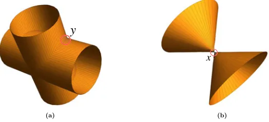
and4.21. The geometry that distinguishes points inMd,G that are also inMd−1,G is illustrated schematically in Figure1.
In what follows, we will make the formal argument as weak as possible, only focusing on generic points, but we will also add remarks as we go along, with stronger statements for geometric intuition.
LEMMA 4.2. Let G be generically locally rigid inCd, with n
> d+1vertices.
Suppose (G,p) is an infinitesimally flexible framework. Then the point x :=
Figure 1. Two types of singular points on ruled varieties. (a) The Gauss fibers on a variety consisting of two intersecting cylinders consist of the ruling lines indicated. Points in the intersection of the two cylinders, such as the one markedyare in the singular locus, but still lie in the closure of a finite number of generic Gauss fibers (in this case, one ruling line from each cylinder). Proposition4.20says that measurementsythat arise from configurations with full spans are either smooth points (in a single fiber closure) or lie in the closure of a finite number of generic Gauss fibers as in this figure. (b) The Gauss fibers on the elliptic cone also consist of ruling lines, as indicated. The cone point, marked asx, lies in the closure of an infinite number of ruling lines. This is a different situation than we saw (fory) in (a). Proposition4.21says that measurementsxthat arise from configurations with deficient spans lie in the closure of an infinite number of generic Gauss fibers as in this figure.
In particular, ifphas deficient affine span, then mG(p)is nongeneric.
Proof sketch. From Theorem 2.10, G is generically locally rigid if and only if
it is generically infinitesimally rigid if and only if the generic dimension of the differential ofmG(·)isdn− d
+1 2
.
Ifxis not a smooth point ofMd,G then it cannot be generic and we are done. Next we restrict the mapmG(·)by removing the nonsmooth points fromMd,G and then removing the preimages of these nonsmooth points from the domain. By assumption, the configurationpis not a regular point ofmG(·), makingxnot a regular value of its image.
But from Sard’s theorem applied tomG(·), the set of critical values is of lower dimension. This set is also constructible and defined overQ. This set remains of
lower dimension under closure, thus the critical values must satisfy some extra equation, making them nongeneric.
DEFINITION4.3. FixdandG. We say thatxis anunhitpoint ofMd,Gif there is no configurationpsuch thatx=mG(p). Otherwise it ishit.
LEMMA4.4. Let G be an ordered graph on n>d+1vertices that is generically
locally rigid in Cd. Let x be generic in Md,G. Then x is hit. Moreover, any
configurationphittingxis infinitesimally rigid and has full affine span.
Proof. The hit set is an irreducible constructible set withMd,G as its closure. By
LemmaA.4, it must then contain a nonempty (Zariski) open subset ofMd,G. Thus the unhit set must be contained in a closed subset (that is, a subvariety). This renders all unhit points nongeneric.
Infinitesimal rigidity follows from Lemma4.2, which also gives us the stated span.
DEFINITION 4.5. Letp be a configuration inCd with a full affine span. Then
theopen affine classA(p)is the set of configurations that are affine images ofp, and are nondegenerate (have full span). An affine class isgeneric if it contains a generic configuration. (Generic affine classes exist, sinceA(p)is defined for everypwith full span.)
Given a generic affine classA, we define the generic locusAgto be the subset of configurations inAthat are also generic as configurations.
LetA(p)be the closure of an affine class. This includes the degenerate affine images.A(p)is a linear space.
LEMMA4.6. Let G be an ordered graph on n vertices andpa configuration of n
points inCd. Then mG(A(p))is a linear space, and in particular, it is closed.
Proof. For each edgei j ofG, define its edge vector ase:=pi−pj inCd. Then
the complex squared length on that edge is the vector productete.
An affine transform,A, applied topcan be expressed aspi →Mpi+t, where
Mis somed-by-d complex matrix andtis some (translation) vector. The effect on each edge vector is of the formei j → Mei j. The effect on its squared length isete→etMtMe=:etQe=tr(Qeet), whereQis a symmetric matrix. Note that the rightmost expression is linear inQ.
Since we are in the complex setting, using a Takagi factorization, every symmetric matrixQarises in this form from someM.
Thus, we can model the action ofmG(·)onA(p)by defining a mapnG,p(Q) from symmetricd×dmatricesQtoCm that acts coordinate-wise asn
DEFINITION 4.7. Let V be an irreducible homogeneous variety. We define an
(open) Gauss fiber F of V to be a maximal set of smooth points of V with a
common tangent space. (For an inhomogeneous variety, we would instead have to work with affine tangent planes.) We say that F is ageneric Gauss fiberif it contains a point that is generic inV. Given a generic Gauss fiber F of V, we define the generic locus Fg to be the subset of points in F that are also generic inV.
The term ‘Gauss fiber’ is used as it is the fiber above a point in the image
of the (rational) Gauss map x 7→ TxV, taking each smooth point of V to the
appropriate Grassmanian. Importantly, the definitions of F andFg only depend on the geometry of the varietyV, and not on any other information (such as how
V may have been generated from some graph).
REMARK 4.8. A deeper result about ruled varieties states that if F is a generic Gauss fiber of any irreducible homogeneous variety, then its closure,F, is always a linear space [8, Section 2.3.2], and in particular, irreducible. This also tells us thatFg is dense inF(LemmaA.6) and soFg= F.
The next set of lemmas will establish a correspondence between generic Gauss fibers ofMd,G and affine classes of configurations.
DEFINITION4.9. LetVbe a homogeneous variety inCm. Letxbe a smooth point
inV. Letφbe a nonzero element of(Cm)∗
. We say thatφistangenttoV atxif TxV ⊆ker(φ). We will call (with slight abuse of duality) such aφatangential
hyperplane.
The following lemma relates an equilibrium stress vector for (G,p) to the geometry ofMd,G aroundmG(p).
LEMMA 4.10 [13, Lemma 2.21]. Let G be an ordered graph with n > d +2
vertices. Let(G,p)be an infinitesimally rigid framework with mG(p)smooth in
Md,G (such as whenp is generic). A nonzeroω ∈ (Cm)∗ is tangent to Md,G at
mG(p)if and only ifωis an equilibrium stress for(G,p).
LEMMA4.12. Let G, an ordered graph on n >d+2vertices with m edges, be
generically globally rigid inCd. Let F be a generic Gauss fiber of Md,G. Then
there exists a single affine classAsuch that allpwith mG(p)∈Fgare inA; that is, m−G1(Fg)⊆A. This classAis generic.
Proof. From Lemma4.4, eachx∈Fgis hit, giving us at least onepwithm
G(p)=
x. Also from Lemma4.4, each suchpis infinitesimally rigid and thus has a full span.
Lemma4.10then tells us that the equilibrium stresses for(G,p)withmG(p)∈ Fg correspond to the tangential hyperplanes atm
G(p). Since the tangents, and thus tangential hyperplanes, agree for allx∈Fg, all suchpshare the same space Sof equilibrium stresses.
From LemmaA.8, above anyx∈Fgthere is a generic configurationqand from Theorem2.15 (see also Remark2.16)qhas a shared stress kernel of dimension
d+1. ThusSmust have a shared stress kernel of dimensiond+1. This makes
the dimension of the set ofd-dimensional configurations having this stress space S equal tod(d+1). In particular, this places all suchpin some unique closed affine classA¯. This, along with the established affine span of pplaces it inA. Genericity ofAcomes from the genericity ofq.
In light of Lemma4.12, the following is well defined.
DEFINITION4.13. LetG, an ordered graph onn>d+2 vertices withmedges, be generically globally rigid inCd. LetFbe a generic Gauss fiber ofMd,G. Define, by an overloading of notation,A(F)to be the generic affine classA(p)for any/every
pabove any x ∈ Fg. We also denote by A(·) the map F 7→ A(F), which is defined for generic Gauss fibers ofMd,G.
REMARK4.14. From Remark4.11, whenGis generically globally rigid andqis any configuration so thatmG(q)is smooth and in a generic Gauss fiber F(even ifmG(q)is not in Fg), thenq ∈A(F). Additionally, any suchqmust have an equilibrium stress matrix of rankn−d −1. If additionally, qhas a full affine span, thenq∈A(F). (Later we will see that suchq, withmG(q)smooth, must in fact always have full affine span.)
LEMMA 4.15. Let G, an ordered graph on n > d+ 2vertices with m edges,
be generically globally rigid inCd. If p1 andp2 are generic configurations and
A(p2) = A(p1), then m
G(p1) and mG(p2) are both generic and in the same
generic Gauss fiber of Md,G. Thus, if F1and F2are two different generic Gauss
Proof. We proceed as in the proof of Lemma 4.12. Since p1 and p2 are nonsingular affine images of each other, they must satisfy all of the same equilibrium stress matrices. Thus mG(p1) and mG(p2) must have the same
tangential hyperplanes, and be in the same Gauss fiber F of Md,G. From
LemmaA.7, the imagesmG(pi),i = 1,2 are generic, so F is a generic Gauss fiber.
We get the following corollary, which is also interesting in its own right.
PROPOSITION 4.16. Let G, an ordered graph on n > d +2 vertices with m
edges, be generically globally rigid inCd. The mapA(·)gives a bijection between
generic Gauss fibers of Md,G and generic affine classes. Finally, we have Fg =
mG(A(F)g).
Proof. Lemma4.15implies that the mapA(·)from generic Gauss fibers ofMd,G
to affine classes is injective. LemmaA.8also implies that ifFis a generic Gauss fiber ofMd,G thatA(F)is a generic affine class.
The mapA(·)is also surjective. By definition, a generic affine class arises as
A(p)for a generic configurationp. By LemmaA.7, the imagemG(p)is generic inMd,G. Hence the Gauss fiber containingmG(p)is generic. SinceA(p)was an arbitrary generic affine class, we have surjectivity.
From Lemma4.12we havem−G1(Fg)⊆ A(F). Since, from Lemma4.4, each point inFg is hit, this gives us Fg ⊆ m
G(A(F)). From LemmaA.8, this means
Fg ⊆m
G(A(F)g).
In the other direction, Lemma 4.15 gives us F ⊇ mG(A(F)g). From
LemmaA.7, this meansFg ⊇m
G(A(F)g).
The following is the main structural lemma that we will need going forward.
LEMMA4.17. Let G, an ordered graph on n >d+2vertices with m edges, be
generically globally rigid inCd. Let F be a generic Gauss fiber of M
d,G. Then
Fg =m
G(A(F)).
Proof. From Proposition4.16we haveFg =m
G(A(F)g)⊆mG(A(F)).
From LemmaA.6, A(F)g is dense in A(F) and soA(F)g = A(F). From continuity, we have mG(A(F)g) ⊇ mG(A(F)g). Thus Fg = mG(A(F)g) ⊇ mG(A(F)g)=mG(A(F)).
For the other direction, we have established above that Fg ⊆ m
REMARK4.18. In light of Remark4.8, we see that for a generically globally rigid graphG and generic Gauss fiberF of Md,G, we actually have F = mG(A(F)). This also means that all points of Fare hit.
LEMMA4.19. Let G, an ordered graph on n >d+2vertices with m edges, be
generically globally rigid inCd. Letxbe any point (not necessarily generic) in
Md,G \Md−1,G and in Fg, for some generic Gauss fiber F of Md,g. There must
be a configurationqthat has full span and is inA(F)such that mG(q)=x. For
such aq, the framework (G,q)must be infinitesimally rigid, and hence also be
locally rigid.
Proof. From Lemma4.17there must be someqinA(F)such thatmG(q)= x.
From the assumption thatxis not inMd−1,G, we know thatqmust have an affine span of dimensiond. ThusA(q)is well defined and is equal toA(F).
If(G,q)were infinitesimally flexible, then from Lemma2.6so too would all of the points in A(q), which equals A(F). But from Lemma 4.2, this would contradict the assumed genericity ofF. Local rigidity follows from infinitesimal rigidity and Theorem2.5.
The next two propositions form the central part of our argument. Informally, they say that we can distinguish between points in the measurement set that arise from lower-dimensional configurations from those that are merely singular by looking at the generic Gauss fibers going through them. Figure1gives a schematic of the two situations.
PROPOSITION4.20. Let G be an ordered graph with n > d+2vertices that is
generically globally rigid inCd. Letxbe any point (not necessarily generic) in
Md,G \Md−1,G. Then there are at most a finite number of generic Gauss fibers F of Md,G withxin Fg.
Note that ifxis a smooth point ofMd,Gthen it is in a single generic Gauss fiber closure. But here, we are not making such assumptions onx; for example, we will allow forxthat are measurements of frameworks that are (due to nongenericity) not globally rigid. This can occur even in a generic affine class [6, Example 8.3].
contradict the fact that, up to congruence, there can only be a finite number of locally rigid configurations with the same edge lengths.
Proof of Proposition4.20. Let {Fi|i ∈ I} be the collection of generic Gauss
fibers of Md,G containingxin their closures. A priori, the index set I might be infinite. For every suchFi, from Lemma4.19, there must be a configurationqiin
A(Fi)that has full span, is locally rigid and such thatm
G(qi)=x. Sinceqhas full affine span,A(qi)is well defined and is equal toA(Fi). From Lemma4.15, for any two such distinctFiandFj, we haveA(qi)6=A(qj). Thusqicannot be congruent toqj.
Suppose there were an infinite number of Fi. Then there would be an infinite number of locally rigid congruence classes[qi]that map tox. But this contradicts
Lemma2.8.
PROPOSITION4.21. Let G, an ordered graph on n>d+2vertices with m edges, be generically globally rigid inCd. There is an x, generic in Md−1,G, such that there are an infinite number of Gauss fibers F of Md,G withxin Fg.
The key idea is that ifqis a configuration with a deficient affine span, then there are an infinite number of configurationspwith full affine spans such that
q∈A(p). This will give us an infinite number of generic Gauss fibers withx= mG(q)in their closures.
Proof. We start with a generic configuration p. Let π be the projection from
d-dimensional configurations to d − 1 dimensional configurations that simply
ignores the last spatial coordinate. Letq := π(p)and x :=mG(q). Since pis generic as ad-dimensional configuration,qis generic as a(d−1)-dimensional configuration, andxis generic inMd−1,G.
LetFbe the Gauss fiber of Md,G that containsmG(p). Sinceq∈A(F), from Lemma4.17,xis in Fg. This gives us one fiberF for the proposition. Now we show how to get more.
DefineL(p):= π−1(q)to be the space of lifts ofq. The space of lifts is an affine space that containsp, and so, by LemmaA.6,L(p)contains a dense set of generic configurations. Sincen>d+2, we can find an infinite number ofp0that
are generic configurations, are inL(p)and with each in a different affine class. (Any finite number of affine classes are contained in a finite number of strict subvarieties of the linear lifting space, and thus cannot cover all of the generic configurations.)
For any such configuration, sayp0
, that is not inA(p), we can apply the same argument to get another Gauss fiberF0
F 6= F0
. Since we can do this endlessly, we obtain our infinite number of fibers forx.
REMARK 4.22. Anyxmeeting the hypotheses of Proposition4.21 cannot be a smooth point in Md,G (as it is in the closure of multiple Gauss fibers, and the Gauss map, where defined, is continuous). Since thisxis also generic inMd−1,G, we can conclude that all ofMd−1,G lies in the singular locus ofMd,G.
REMARK4.23. To recap, everyqwithmG(q)smooth and in a generic Gauss fiber Fof a generically globally rigid graphG, has a full affine span, is infinitesimally rigid, and is inA(F). Such a framework(G,q)must be globally rigid [5].
The closure of Fis the linear space mG(A(F)). This means that all points in Fare hit. It also means that, for each pointx∈F, there must be some pointqin
A(F)withmG(q)=x.
Points that are smooth inMd,G are in only one Gauss fiber and one Gauss fiber closure.
LetFbe a generic Gauss fiber. Let the ‘bad’ points beB:= F\F. These are nonsmooth inMd,G. Points that are inBdue to deficient span will, generically, be in the closure of infinitely many distinct generic Gauss fibers. All ‘other’ points inB(no deficient span in the preimage) can be in only a finite number of generic F. (Any of the preimagesqof these other bad points is also infinitesimally rigid.) These other bad points can occur, say, when(G,q)is not globally rigid. (Note that global rigidity of frameworks is not an affine invariant property [6, Example 8.3].) At nongeneric Gauss fibers F of Md,G, most bets are off. F can be of some larger dimension, and conceivably be reducible. It is even conceivable that there areqthat have full spans and are infinitesimally flexible but such thatmG(q)is still a smooth point ofMd,G (in such a nongenericF).
The next lemmas will let us treat G and H symmetrically. We start with a
technical result about Gauss fiber dimension that allows us to identify generic global rigidity intrinsically inMd,G.
LEMMA4.24. Let G be a generically locally rigid graph with n>d+2vertices
and m edges. Suppose that, at some genericpthe shared stress kernel of(G,p)
has dimension k > d +1. Let F be the Gauss fiber of Md,G containing mG(p).
Then the dimension of Fgis dk− d+1
2
.
Proof. Let p be a generic configuration. Define K to be the space of
configurations q such that (G,q) satisfies all the equilibrium stresses (G,p)
As discussed in Definition2.14, k, the dimension of the shared stress kernel, is at least d +1. Hence, K is of dimension at leastd(d +1). Moreover (see Definition2.13) K must include all affine images ofp, including all qthat are congruent top.
LetKgbe the configurations inK that are generic in configuration space. From LemmaA.6,Kgis a dense subset ofK, which is closed, and soKg= K.
LetFbe the Gauss fiber ofMd,GcontainingmG(p);Fis generic becausepis.
Now that we know F is a generic affine class, we can show that Fg = m
G(Kg) by following the proof of the same statement in Proposition4.16. This gives us
Fg =m
G(Kg)=mG(Kg)=mG(K). The second equality is due to continuity. From the above, we get dim(Fg)=dim(m
G(K))=dim(mG(K)). The second equality is due to the fact that a constructible set and its Zariski closure have the same dimension. (In the case thatGis generically globally rigid, thenK =A(F)
and due to Lemmas4.6and4.17we actually haveFg=m
G(K).)
By generic local rigidity of G, we know that the maximum rank of dmG,
restricted to its action on K, is dk − d+1
2
. (Recall that K includes all
configurations that are congruent to p. It follows that, at p, the differential ofmG, acting as a map restricted toK, has a kernel of dimension at least
d+1 2
, corresponding to the trivial infinitesimal flexes. If this kernel at our generic p
were any larger,(G,p)could not be infinitesimally rigid.)
Using the constant rank theorem and Sard’s Theorem as in the proof of Lemma3.3, we conclude that the dimension ofFgis exactly this size.
REMARK4.25. Using the fact that, in fact,Fis irreducible (see Remark4.8), we can improve Lemma4.24to give the dimension ofFinstead of Fg.
We now interpret Lemma4.24in terms of generic global rigidity.
LEMMA4.26. Let G, an ordered graph on n >d+2vertices with m edges, be
generically globally rigid inCd. Let H be some ordered graph also with n vertices
with m edges. Suppose Md,G = Md,H. Then H is also generically globally rigid
inCd.
Proof. SinceMd,G = Md,H, they, in particular have the same dimension. IfG is
generically globally rigid, then it is also generically locally rigid. By Lemma3.3
this implies thatH (having the same number of vertices asG) is also generically locally rigid.
BecauseMd,GandMd,Hare the same variety, the generic Gauss fiberFofMd,G containingx:=mG(p)is also the generic Gauss fiber of Mx,H containingx(and
Lemma4.24then lets us compute the dimension of Fg in two different ways, using the shared stress kernel of (G,p) and (H,p), respectively. Since G is generically globally rigid, Theorem2.15implies its shared stress kernel is(d+1) -dimensional. To avoid a contradiction from Lemma4.24,(H,p)must also have a shared stress kernel of dimensiond+1, in which case Theorem2.15implies that H is also generically globally rigid.
With all this in hand, we can complete the proof of the main proposition of this section.
Proof of Proposition4.1. From Proposition 4.21, there is a point x generic in
Md−1,G in an infinite number of Fg. From Lemma 4.26 and Proposition 4.20,
x must also be in Md−1,H. Since x is generic, this implies that Md−1,G ⊆ Md−1,H (otherwise the equations ofMd−1,H would certifyxas nongeneric). From
Lemma4.26we can apply the same argument in the other direction to conclude
Md−1,H ⊆ Md−1,G.
For the induction, we use Lemma2.11.
5. d=1
In this section, we prove the following proposition:
PROPOSITION5.1. Let G and H be ordered graphs, with>3vertices. Suppose
that G is3-connected, H has no isolated vertices, and M1,G = M1,H. Then there
is a vertex relabeling under which G= H .
This establishes the base case for an inductive proof of Theorem3.4, which we prove at the end of the section.
DEFINITION5.2. LetV ⊆CN be an irreducible affine variety. Let Lbe a linear subspace. LetπLdenote the quotient map takingCN toCN/L.
Let[N] = {1, . . . ,n}. For eachI ⊆ [N]thecoordinate subspace SIis the linear
span of the coordinate vectors indexed byI; that is,SI =lin{ei :i ∈ I}. Define I := [N] \I for I ⊆ [N]. A coordinate subspaceSI isindependentinV if the dimension ofπSI(V)is|I|. OtherwiseSI isdependentinV.
LEMMA5.3. Let E0
be the subset of the edges of G. SE0is independent in M1,G if and only if the edges of E0
Proof. If E0
is a forest, then given any target measurement values in C|E
0| , we can traverse the forest and sequentially place the vertices inC1 to achieve this
measurement. Conversely, if E0
is not a forest, then it contains a cycle C. The sum of the vectors connecting the points ofC inC1must sum to zero, giving us a nontrivial
equation that must be satisfied.
DEFINITION 5.4. A subset of edges E0
of a graph G is cycle supportedif the edges ofE0, in some order, form a simple cycle in
G. An edge bijectionσbetween two graphsG andH, is acycle isomorphismif it maps cycle supported sets, and only cycle supported sets, to cycle supported sets.
LEMMA 5.5. Let G and H be ordered graphs with m edges. Suppose M1,G =
M1,H. Then the mapping taking the ordered edges of G to the ordered edges of H
is a cycle isomorphism.
Proof. Suppose the mapping is not a cycle isomorphism. Then without loss of
generality, there is a set of edgesCthat form a simple cycle inGand notH.
Suppose that this C forms a forest in H. Then from Lemma 5.3, we have
πSC(M1,G)6=πSC(M1,H)and thusM1,G 6=M1,H.
Suppose instead that thisC is neither a simple cycle nor a forest in H, then there must be an edgeesuch thatC0:=
C −eis not a forest in H, whileC0
is a forest inG(a simple cycle minus one edge is a path). Then from Lemma5.3, we haveπSC0(M1,G)6=πSC0(M1,H)and thusM1,G 6=M1,H.
A theorem of Whitney [30] (see also [26]) allows us to upgrade cycle
isomorphisms to graph isomorphisms.
THEOREM5.6. Let G and H be two graphs, with G being3-connected, and H with no isolated vertices. An edge bijection that is a cycle isomorphism must arise from a graph isomorphism.
REMARK 5.7. Another way to state Whitney’s theorem is that ifG andH have
isomorphic graphic matroids and no isolated vertices, and G is 3-connected,
then G and H are isomorphic as graphs. In particular, topological information
contained in the ordering of the edges on a cycle is not part of the hypothesis, nor did we consider it in Lemma5.5.
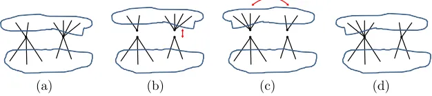
Figure 2. The reversal operation. The graphs, (a) and (d) are 2-isomorphic but not isomorphic. Note that the edge lengths of the frameworks are unchanged under a 2-isomorphism.
REMARK 5.8. If G is not 3-connected, then there are cycle isomorphisms
betweenG and nonisomorphic H. Whitney [31] showed that these belong to a
restricted class of ‘1-isomorphisms’ and ‘2-isomorphisms.’ See Figure2for an example of a pair of 2-isomorphic graphs.
With this in hand, we can prove the main proposition of this section.
Proof of Proposition5.1. From Lemma 5.5the mapping taking the edges ofG
to H must be a cycle isomorphism. Then from the assumed 3-connectivity and
Theorem5.6this mapping must arise from a vertex relabeling.
The main structural theorem of this paper now follows.
Proof of Theorem3.4. From Proposition4.1we can reduce the problem from d
dimensions down to 1. SinceGis generically globally rigid ind>2 dimensions, from Theorem2.12it must be 3-connected. Since the number of vertices in both graphs is the same andM1,G = M1,H, from Lemma3.3, H cannot have isolated vertices. The result then follows from Proposition5.1.
As proven in the end of Section3, this immediately proves the main result of this paper, Theorem1.5.
6. Bonus result
DEFINITION6.1. Letdbe some fixed dimension andna number of vertices. Let G := {E1, . . . ,Em}be an ordered graph. The ordering on the edges ofG fixes an association between each edge inGand a coordinate axis ofRm.
We denote by ME
d,G the image of mEG(·) over all real d-dimensional
configurations. We call this the (squared) Euclidean measurement set of G
(inddimensions). This is a real semialgebraic set, defined overQ.
THEOREM 6.2. Let d be fixed. Let G be an ordered 3-connected graph on n vertices with m edges, and H some ordered graph with no isolated vertices and
with m edges. Suppose ME
d,G = MdE,H. Then there is a vertex relabeling of H such
that G= H .
REMARK 6.3. This theorem does not rule out the possibility that there are two
nonisomorphic graphs G and H such that ME
d,G ∩ MdE,H contains a standard-topology open set. This would imply that Md,G is equal to Md,H even though
ME
d,G 6=MdE,H. In this case, there could be some generic Euclidean measurements that are achievable from both graphs and some generic Euclidean measurements that are achievable only in one graph.
As a result, Theorem6.2does not help us to prove Theorem1.5.
The rest of this section proves Theorem6.2. The steps are similar to the ones we used in Section5, but in the present setting, they work immediately in dimensions greater than one.
LEMMA6.4. Let E0be the subset of the edges of G.πSE0(M
E
d,G)equals the entire first octant if and only if the edges of E0
form a forest over the vertices of G.
Proof. If E0 is a forest, then given any target measurements point in the first
octant ofR|E
0|
, we can traverse the forest and sequentially place the vertices inRd
to achieve this measurement.
Conversely, ifE0is not a forest, then it contains a cycle
Conkedges, for some k. In this case,πSE0(M
E
d,G)cannot be the entire first octant ofR
ksince there is no
real framework (in any dimension) where all but one of the edges of the cycle has zero length.
LEMMA 6.5. Let G and H be ordered graphs with m edges. Suppose ME
d,G =
ME
d,H. Then the mapping taking the ordered edges of G to the ordered edges of H
Proof. Suppose the mapping is not a cycle isomorphism. Then without loss of generality there is a set of edgesC that from a simple cycle inG and notH.
Suppose thatC is a forest in H. Then from Lemma6.4, we haveπSC(M E d,G)6=
πSC(MdE,H)and thusMdE,G 6=MdE,H.
Suppose thatCis neither a simple cycle nor a forest inH, then there must be an edgeesuch thatC0:=
C −eis not a forest inH, whileC0is a forest in
G. Then from Lemma6.4, we haveπSC0(M
E
d,G)6=πSC0(M
E
d,H)and thusMdE,G 6=MdE,H.
Proof of Theorem6.2. The theorem now follows directly from Lemma6.5, the
assumed 3-connectivity, and Theorem5.6.
7. Remaining issues
This paper answers some central questions about the relationships between graphs and their measurement varieties/sets. There are a few natural remaining questions.
7.1. Redundant rigidity. Theorem 1.5is tight in the sense that if G is not generically globally rigid ind dimensions, then clearly we cannot determinep
fromv. But it is still possible that one might be able to determineGfromv. Here we discuss a possible strengthening of Theorem3.4.
DEFINITION7.1. We say that a graphG isgenerically redundantly rigidinRdif
Gis generically locally rigid inRdand remains so after the removal of any single edge.
QUESTION7.2. Is the following claim true:
Let G, an ordered graph with n>d+2vertices and m edges, be3-connected
and generically redundantly rigid in d dimensions. Let H be some ordered graph
on n vertices with m edges. Suppose Md,G = Md,H. Then there is a vertex
relabeling under which G= H .
The claim is true ford = 2, since in two dimensions, redundant rigidity and 3-connectivity imply generic global rigidity [5,18].
In terms of the ingredients used for proving Theorem 3.4, we note that the conclusion of Proposition4.20is false whenGis merely generically redundantly rigid. For example the complete bipartite graph,K5,5, is redundantly rigid in three
dimensions and is 4-connected. But for any configurationqwhere even one of
Figure 3. A pair of nonisomorphic graphs with the same measurement variety. Any of the green edges in the graphs (a) and (b), if removed, result in a graph that is generically flexible. As described in Remark7.4, these graphs have the same measurement variety (it is the product of the measurement varieties of the complete graph K4, the wheel W4 andC3). However, the graphs (a) and (b) are
not isomorphic, because the dashed green edges can be distinguished from each other by the degree of the endpoint on the right.
fibers withmG(q)in their closure. This is because equilibrium stresses for generic
p, which are all rank 2, only enforce affine relations within each of the parts [3].
A positive answer to Question7.2would directly imply Theorem3.4due to
Theorem2.12and the following theorem of Hendrickson [16].
THEOREM7.3. If G is generically globally rigid inRd, with n>d+2then it is
redundantly rigid inRd.
REMARK7.4. A positive answer to Question7.2would give us a reasonably tight characterization of measurement variety agreement in light of the following.
Suppose that G is not generically redundantly rigid, and let e be an edge of G so thatG0:=
G−e is generically locally flexible. From the size ofG, there must be a nonedgee0
ofG different fromewhose lengths can be changed under
a continuous flex ofG0. Let
G00 be the graph obtained from
G by replacinge
withe0
. ThenMd,G = Md,G00 as both are equal toMd,G0⊕C1. (See an example in Figure3.) But the mapping fromG toG00
will not be an isomorphism for graphs unlesse ande0 are in the same orbit of Aut(
G +e0). This is a very restrictive
condition onGthat any extension of our results to graphs that are not generically redundantly rigid will have to include. (Garamv¨olgyi and Jord´an [9] explore the question of when a nonredundantly rigid graph can be reconstructed from edge-length measurements.)
There are also some more unresolved issues about measurement sets.
QUESTION 7.5. Can the assumption that G and H have the same number of
more vertices, but is generically locally flexible. Garamv¨olgyi and Jord´an[9]give an affirmative answer in dimensions one and two.)
More generally, we know very little about what assumptions other than dimension can let us conclude for generald thatMd,G ⊆ Md,H implies Md,G = Md,H.
7.2. Unlabeled graph realization. The graph realization (or distance
geometry) problem asks to reconstruct an unknown configuration p given a
graphG, dimensiond, and labeled edge-length measurementsv=mE
G(p). From
Theorem 1.4, if we assume that p is generic and know that G is generically
globally rigid, and we can find any q at all (not necessarily generic) so that
v=mE
G(q), then we know thatq=p(up to congruence). As a practical matter, it is important thatqneed not be generic, since this is a very strong restriction on (or assumption about) any specific algorithm (as opposed to the process generating the inputp).
Theorem1.5does not immediately give us the analogous result forunlabeled
distance geometry. The subtlety is that the hypotheses of Theorem1.5 include
knowledge aboutG, which we will not have access to in an unlabeled distance
geometry instance. Unlike in the labeled case,vby itself does not immediately tell us whether our problem is generically well posed.
Examining our proofs, we get a partial result in this direction:
THEOREM7.6. In any fixed dimension d >2, letpbe a generic configuration of
n>d+2points. Letv=mE
G(p), where G is an ordered graph (with n vertices
and m edges) that is generically locally rigid inRd.
Suppose there is a configurationq, also of n points, along with an ordered
graph H (with n vertices and m edges) that is generically globally rigid and such
thatv=mE
H(q).
Then there is a vertex relabeling of H such that G= H . Moreover, under this
vertex relabeling, up to congruence,q=p.
Proof sketch. The derivation of Theorem 1.5 from Theorem 3.4 works nearly
unmodified. Both G and H are generically locally rigid by hypothesis and so
Md,G andMd,H are of the same dimension. The configurationpmaps to a generic point in the intersection ofMd,G andMd,H, so the two measurement varieties are equal. When applying3.4, we rely on the generic global rigidity of H instead ofG. The rest of the proof then goes through unchanged.
generic global rigidity can be tested in a realization setting) andqcertify that the input problem is, in fact, well posed, and that we have found its solution. This version still makes some assumptions onGand the number of vertices in H.
This motivates the following question.
QUESTION7.7. Is the following claim true:
In any fixed dimension d >2, letpbe a generic configuration of n > d+2
points. Let v = mE
G(p), where G is an ordered graph (with n vertices and m
edges). LetpS be the subconfiguration of pindexed by the vertices within the
support of G.
Suppose there is a configurationq, of n0
points, with no two points coincident,
along with an ordered generically globally rigid graph H (with n0
vertices and m0
edges) such thatv=mE
H(q).
Then there is a vertex relabeling ofpS such that, up to congruence, q = pS.
Moreover, under this vertex relabeling, G= H .
A positive answer to this question would mean that, under the assumption that
pis generic, such an(H,q)would be a certificate that we have correctly realized the measured subconfiguration ofp.
The difficulty for this question is that we do not know how to rule out the possibility thatMd,G (Md,H. This is related to the issues mentioned at the end of Section7.1.
There is one special case of note. The claim of this question is true when H is the complete graphKd+2, (see [10, Proposition 4.23]). This is due to the fact
that, aside from Kd+2, any other graph G with N :=
d+1 2
distinct edges has the property that every subset of edges is independent. Hence, the measurement variety, Md,G, of G must be equal to all of CN, and so it cannot be a subset of Md,H. Applying this idea iteratively, it can be shown that the claim of the question remains true if H allows for trilateration [10]. This fact allows one to apply trilateration to an unlabeled set of measurements, as is done in [20], without any assumptions onG orn.
7.3. Matrix completion. A variant of global rigidity is ‘matrix completion’, which asks whether all the entries of anm ×n matrix Aof (low) rankr can be determined by a subset of its entries (at known positions). (See [28] for complete definitions and background.)
matrix completion, a result of [22] says that whether an observation pattern has a unique completion is a generic property. This means it makes sense to ask whether our results also hold in the matrix completion setting.
The following rank 3 examples are from [23] (a preprint version of [22]).
? ? ? ? ? ? ? ? ? ? ? ? ? ? ? ? ? ?? ? ? ? ?? ? ? ? ?? ? ? ? ? ?? ? ? ? ?? ? ??? ? ? ??? ? ?? ? ? ? ?? ? ? ?
It is shown there that, for each of these, the projection onto the known entries (labeled ‘?’) is dominant. Hence, they both have the same ‘measurement varieties’. Additionally, if the underlying matrix is generic, there is exactly one way to fill in the unknown entries (labeled ‘?’), so they are also ‘globally rigid’.
Importantly, they arenotrelated by row and column permutations, so we have a counterexample to the straightforward translation of our main results to the matrix completion setting. (What goes wrong is that the stress criterion for global rigidity is not necessary for matrix completion. This was first observed in [28].)
On the other hand, as noted in [10, Remark 4.20], the matrix completion
analogue of Boutin and Kemper’s result for complete graphs is straightforward. Clarifying the relationship between unlabeled matrix completion and unlabeled rigidity would be interesting.
Acknowledgements
The authors thank Brian Osserman for fielding algebraic geometry queries, Meera Sitharam for feedback and discussions on the relationship to matrix completion, and Robert Krone for an interesting question about coincident points. The first author was partially supported by NSF grant DMS-1564473.
Appendix A. Algebraic geometry background
DEFINITION A.1. A (complex embedded affine) variety(or algebraic set), V, is a (not necessarily strict) subset of CN, for some N, that is defined by the
simultaneous vanishing of a finite set of polynomial equations with coefficients inCin the variablesx1,x2, . . . ,xNwhich are associated with the coordinate axes ofCN. We say thatV isdefined overQif it can be defined by polynomials with
A variety is homogeneous if its ideal is finitely generated by homogeneous polynomials. This is the same as the setV being a cone with its vertex at 0.
A variety can be stratified as a union of a finite number of complex analytic
submanifolds of CN. A variety V has a well defined (maximal) dimension
Dim(V), which will agree with the largest D for which there is a standard-topology open subset ofV, that is aD-dimensional complex analytic submanifold ofCN.
The set of polynomials that vanish onV form a radical ideal I(V), which is generated by a finite set of polynomials.
A variety V is reducibleif it is the proper union of two varieties V1 and V2. Otherwise it is calledirreducible. A variety has a unique decomposition as a finite proper union of its maximal irreducible subvarieties calledcomponents.
Any (strict) subvarietyW of an irreducible varietyV must be of strictly lower dimension.
A subsetW of a varietyV is calledZariski closedifW is a variety.
DEFINITION A.2. The Zariski tangent space at a point x of a variety V is the kernel of the Jacobian matrix of a set of generating polynomials for I(V) evaluated atx.
A pointxof an irreducible varietyVis called (algebraically)smoothinVif the dimension of the Zariski tangent space equals the dimension ofV. Otherwisexis called (algebraically)singularinV.
A smooth point x in an irreducible variety V has a standard-topology
neighborhood in V that is a complex analytic submanifold ofCN of dimension
Dim(V).
Thelocusof singular points ofV is denoted by Sing(V). The singular locus is
itself a strict subvariety ofV.
DEFINITIONA.3. Aconstructible set Sis a set that can be defined using a finite number of varieties and a finite number of Boolean set operations. We say thatS
isdefined overQif it can be defined by polynomials with coefficients inQ.
S has a well defined (maximal) dimension Dim(S), which will agree with
the largest S for which there is a standard-topology open subset of S, that is a D-dimensional complex analytic submanifold ofCN.
TheZariski closureofSis the smallest varietyV containing it. The set Shas
the same dimension as its Zariski closureV. IfSis defined overQ, then so too is
The image of a varietyV under a polynomial map is a constructible setS. IfV is defined overQ, then so too isS[2, Theorem 1.22]. IfV is irreducible, then so
too is the Zariski closure ofS. (We say thatSisirreducible.)
The following can be found in [24, Proposition 10.1].
LEMMA A.4. An irreducible constructible set S contains a Zariski open subset
of its Zariski closure V . Thus V \S is contained in a subvariety W of V . If S is
defined overQ, there is such a W that is as well.
DEFINITIONA.5. A point in an irreducible variety or constructible set,Vdefined overQis called genericif its coordinates do not satisfy any algebraic equation
with coefficients inQbesides those that are satisfied by every point inV. The set of generic points has full measure inV.
WhenV is an irreducible variety and defined overQ, all of its generic points
are smooth.
A generic real configuration inRd(as in Definition1.2) is also a generic point
inCN, considered as a variety, as in the current definition.
LEMMA A.6. Let V ⊆ W be an inclusion of varieties where W and V are
irreducible and W is defined overQ. Suppose that V has at least one pointy
which is generic in W (overQ). Then the points in V which are generic in W are
Zariski dense in V .
Proof. Letφbe a nonzero algebraic function onW defined overQ. Consider the
Zariski open subset set Xφ := {x ∈ V | φ(x) 6= 0}. This is nonempty due to
our assumption about the pointy. Thus, from the irreducibility ofV, thisXφ is
Zariski dense inV.
The set of points inV which are generic inW is defined as the intersection of these open and denseXφasφranges over the countable set of possibleφ.
WhenU is any Zariski open and dense subset ofV, thenV\U is contained in a strict subvariety ofV. From irreducibility and dimension considerations then,U must contain a standard-topology open and dense subset of the smooth locus ofV. (In fact, using [25, Theorem 1, Page 58], we can see thatU is standard-topology open and dense in all ofV.)
As the smooth locus of V under the standard topology is a Baire space, a