warwick.ac.uk/lib-publications
Manuscript version: Author’s Accepted ManuscriptThe version presented in WRAP is the author’s accepted manuscript and may differ from the published version or Version of Record.
Persistent WRAP URL:
http://wrap.warwick.ac.uk/109455 How to cite:
Please refer to published version for the most recent bibliographic citation information. If a published version is known of, the repository item page linked to above, will contain details on accessing it.
Copyright and reuse:
The Warwick Research Archive Portal (WRAP) makes this work by researchers of the University of Warwick available open access under the following conditions.
Copyright © and all moral rights to the version of the paper presented here belong to the individual author(s) and/or other copyright owners. To the extent reasonable and
practicable the material made available in WRAP has been checked for eligibility before being made available.
Copies of full items can be used for personal research or study, educational, or not-for-profit purposes without prior permission or charge. Provided that the authors, title and full
bibliographic details are credited, a hyperlink and/or URL is given for the original metadata page and the content is not changed in any way.
Publisher’s statement:
Please refer to the repository item page, publisher’s statement section, for further information.
Auxiliary Likelihood-Based Approximate Bayesian
Computation in State Space Models
∗
Gael M. Martin
†, Brendan P.M. McCabe
‡, David T. Frazier
§,
Worapree Maneesoonthorn
¶and Christian P. Robert
kJanuary 9, 2017
Abstract
A new approach to inference in state space models is proposed, using approximate Bayesian computation (ABC). ABC avoids evaluation of an intractable likelihood by matching summary statistics computed from observed data with statistics computed from data simulated from the true process, based on parameter draws from the prior. Draws that produce a ‘match’ between observed and simulated summaries are re-tained, and used to estimate the inaccessible posterior; exact inference being feasible only if the statistics are sufficient. With no reduction to sufficiency being possible in the state space setting, we pursue summaries via the maximization of an auxiliary likelihood function. We derive conditions under which this auxiliary likelihood-based approach achieves Bayesian consistency and show that, in the limit, results yielded by the auxiliary maximum likelihood estimator are replicated by the auxiliary score. In multivariate parameter settings a separate treatment of each parameter dimen-sion, based on integrated likelihood techniques, is advocated as a way of avoiding the curse of dimensionality associated with ABC methods. Three stochastic volatil-ity models for which exact inference is either challenging or infeasible, are used for illustration.
Keywords: Likelihood-free methods, stochastic volatility models, Bayesian consis-tency, asymptotic sufficiency, unscented Kalman filter, α-stable distribution.
JEL Classification: C11, C22, C58
∗This research has been supported by Australian Research Council Discovery Grant No. DP150101728.
The authors would like to thank the Editor, an associate editor and two anonymous referees for very helpful and constructive comments on an earlier draft of the paper.
†Department of Econometrics and Business Statistics, Monash University, Australia. Corresponding
author; email: [email protected].
‡Management School, University of Liverpool, U.K.
§Department of Econometrics and Business Statistics, Monash University, Melbourne, Australia. ¶Melbourne Business School, University of Melbourne, Australia.
kUniversit´e Paris-Dauphine, Centre de Recherche en ´Economie et Statistique, and University of
War-wick.
1
Introduction
The application of Approximate Bayesian computation (ABC) (or likelihood-free
infer-ence) to models with intractable likelihoods has become increasingly prevalent of late,
gaining attention in areas beyond the natural sciences in which it first featured. (See
Beaumont, 2010, Csillery et al., 2010; Marin et al ., 2011, Sisson and Fan, 2011 and
Robert, 2015, for reviews.) The technique circumvents direct evaluation of the likelihood
function by selecting parameter draws that yield pseudo data - as simulated from the
assumed model - that matches the observed data, with the matching based on summary statistics. If such statistics are sufficient, and if an arbitrarily small tolerance is used in
the matching, the selected draws can be used to produce a posterior distribution that is
exact up to simulation error; otherwise, an estimate of the partial posterior - defined as
the density of the unknown parameters conditional on the summary statistics - is the only
possible outcome.
The choice of statistics for use within ABC, in addition to techniques for determining
the matching criterion, are clearly of paramount importance, with much recent research
having been devoted to devising ways of ensuring that the information content of the
chosen set of statistics is maximized, in some sense; e.g. Joyce and Marjoram (2008),
Wegmann et al. (2009), Blum (2010), Fearnhead and Prangle (2012) and Frazier et al.
(2016). In this vein, Drovandi et al. (2011), Gleim and Pigorsch (2013), Creel and
Kristensen (2015), Creelet al.,(2015) and Drovandiet al. (2015), produce statistics via an
auxiliary model selected to approximate the features of the true data generating process.
This approach mimics, in a Bayesian framework, the principle underlying the frequentist
methods of indirect inference (Gouri´eroux et al., 1993, Smith, 1993) and efficient method
of moments (Gallant and Tauchen, 1996) using, as it does, the approximating model to
produce feasible inference about an intractable true model. Whilst the price paid for
the approximation in the frequentist setting is a possible reduction in efficiency, the price
paid in the Bayesian case is posterior inference that is conditioned on statistics that are
not sufficient for the parameters of the true model, and which amounts to only partial inference as a consequence.
Our paper continues in this spirit, but with focus given to the application of auxiliary
model-based ABC methods in the state space model (SSM) framework. Whilst ABC
methods have been proposed in this setting (inter alia, Jasraet al.,2010, Deanet al., 2014,
Martinet al., 2014, Calvet and Czellar, 2015a, 2015b, Yildirimet al., 2015), such methods
use ABC principles (without summarization) to estimate either the likelihood function or
the smoothed density of the states, with established techniques - for example, maximum
likelihood or (particle) Markov chain Monte Carlo (PMCMC) - then being used to conduct
of this literature, including existing theoretical results, as well as providing comprehensive computational insights.)
Our aim, in contrast, is to explore the use of ABC alone and as based on
summariza-tion via maximum likelihood estimasummariza-tion (MLE) of the parameters of an auxiliary model.
Drawing on recent theoretical results on the properties of MLE in misspecified SSMs (Douc
and Moulines, 2012) we provide a set of conditions that ensures that auxiliary
likelihood-based ABC is Bayesian consistent in the state space setting, in the sense of producing
draws that yield a degenerate distribution at the true vector of static parameters in the
(sample size) limit. Use of maximum likelihood to estimate the auxiliary parameters also
allows the concept of asymptotic sufficiency to be invoked, thereby ensuring that - for
large samples at least - maximum information is extracted from the auxiliary likelihood in producing the summaries.
We also illustrate that to the order of accuracy that is relevant in establishing the
theoretical properties of an ABC technique, a selection criterion based on the score of the
auxiliary likelihood - evaluated at the maximum likelihood estimator (MLE) computed
from the observed data - yields equivalent results to a criterion based directly on the
MLE itself. This equivalence is shown to hold in both the exactly and over-identified
cases, and independently of any positive definite weighting matrix used to define the two
alternative distance measures, and implies that the proximity to asymptotic sufficiency
yielded by using the auxiliary MLE in an ABC algorithm will be replicated by the use of
the auxiliary score. Given the enormous gain in speed achieved by avoiding optimization of the auxiliary likelihood at each replication of ABC, this is a critical result from a
computational perspective.
Finally, we briefly address the issue of dimensionality that impacts on ABC techniques
in multiple parameter settings. (See Blum, 2010, Fearnhead and Prangle, 2012, Nott et
al ., 2014 and Biau et al., 2015). Specifically, we demonstrate numerically the improved
accuracy that can be achieved by matching individual parameters via the corresponding
scalar score of the integrated auxiliary likelihood, as an alternative to matching on the
multi-dimensional score statistic as suggested, for example, in Drovandi et al. (2015).
We illustrate the proposed method in three classes of model for stochastic return
volatil-ity. Two of the classes exemplify the case where the transition densities in the state process have a representation that is either challenging to embed within an exact algorithm or is
unavailable analytically. The third class of model illustrates the case where the conditional
density of returns given the latent volatility is unavailable. Satisfaction of the sufficient
conditions for Bayesian consistency of ABC (up to identification conditions) is
demon-strated for one class. Examples from all three classes are then explored numerically, in
artificial data scenarios, with consistent inference being confirmed. This being the first
in such complex settings, the results augur well for the future use of the method.
The paper proceeds as follows. In Section 2 we briefly summarize the basic principles
of ABC as they would apply in a state space framework. In Section 3, we then proceed
to demonstrate the theoretical properties of the auxiliary likelihood approach to ABC,
including sufficient conditions for Bayesian consistency to hold, in this particular setting.
The sense in which inference based on the auxiliary MLE is replicated by inference based
on the auxiliary score is also described. In Section 4 we then consider the application of the
auxiliary likelihood approach in the non-linear state space setting, using the three classes
of latent volatility models for illustration. Numerical accuracy of the proposed method, as
applied to data generated artificially from the Heston (1993) square root volatility model,
is then assessed in Section 5.1. Existence of known (non-central chi-squared) transition densities means that the exact likelihood function/posterior distribution is available for
the purpose of comparison. The accuracy of the auxiliary likelihood-based ABC posterior
estimate is compared with: 1) an ABC estimate that uses a (weighted) Euclidean metric
based on statistics that are sufficient for an observed autoregressive model of order one
defined on the logarithmic squared returns; and 2) an ABC estimate that exploits the
dimension-reduction technique of Fearnhead and Prangle (2012), applied to this latter
set of summary statistics. The auxiliary likelihood-based method is shown to provide
the most accurate estimate of the exact posterior in almost all cases documented. In
Section 5.2 numerical evidence supports Bayesian consistency for the auxiliary-likelihood
based method in all three SSMs investigated in the paper. In contrast, evidence for the consistency of various summary-statistic based ABC methods is mixed. Section 6
concludes. Technical proofs and certain computational details are included in appendices
to the paper.
2
Auxiliary likelihood-based ABC in state space
mod-els
2.1
Outline of the basic approach
The aim of ABC is to produce draws from an approximation to the posterior distribution of
a vector of unknowns, θ, given theT-dimensional vector of observed data y= (y1, ..., yT)0,
p(θ|y)∝p(y|θ)p(θ),
in the case where both the prior, p(θ), and the likelihood, p(y|θ), can be simulated.
These draws are used, in turn, to approximate posterior quantities of interest, including
marginal posterior moments, marginal posterior distributions and predictive distributions.
The simplest (accept/reject) form of the algorithm (Tavar´e et al., 1997, Pritchard, 1999)
Algorithm 1 ABC accept/reject algorithm
1: Simulate θi,i= 1,2, ..., N, from p(θ)
2: Simulate zi = (zi
1, zi2, ..., zTi)
0, i= 1,2, ..., N, from the likelihood, p(.|θi
)
3: Select θi such that:
d{η(y), η(zi)} ≤ε, (1)
whereη(.) is a (vector) statistic,d{.}is a distance criterion, and, givenN, the tolerance level ε is chosen to be small.
The algorithm thus samples θ and zfrom the joint posterior:
pε(θ,z|η(y)) =
p(θ)p(z|θ)Iε[z]
R
Θ
R
zp(θ)p(z|θ)Iε[z]dzdθ
,
where Iε[z]:=I[d{η(y), η(z)} ≤ε] is one if d{η(y), η(z)} ≤ε and zero else. Clearly, when
η(·) is sufficient and ε arbitrarily small,
pε(θ|η(y)) =
R
zpε(θ,z|η(y))dz (2)
approximates the exact posterior, p(θ|y), and draws from pε(θ,z|η(y)) can be used to
estimate features of that exact posterior. In practice however, the complexity of the models
to which ABC is applied, including in the state space setting, implies that sufficiency is
unattainable. Hence, as ε → 0 the draws can be used to estimate features of p(θ|η(y))
only.
Adaptations of the basic rejection scheme have involved post-sampling corrections of
the draws using kernel methods (Beaumont et al., 2002, Blum, 2010, Blum and Fran¸cois,
2010), or the insertion of Markov chain Monte Carlo (MCMC) and/or sequential Monte
Carlo (SMC) steps (Marjoramet al., 2003, Sissonet al., 2007, Beaumontet al., 2009, Toni
et al., 2009, and Wegmann et al., 2009), to improve the accuracy with which p(θ|η(y)) is
estimated, for any given number of draws. Focus is also given to choosingη(.) and/or d{.}
so as to renderp(θ|η(y)) a closer match top(θ|y), in some sense; see Joyce and Marjoram
(2008), Wegmann et al., Blum (2010) and Fearnhead and Prangle (2012). In the latter
vein, Drovandi et al. (2011) argue, in the context of a specific biological model, that the
use ofη(.) comprised of the MLEs of the parameters of a well-chosen approximating model,
may yield posterior inference that is conditioned on a large portion of the information in
the data and, hence, be close to exact inference based on p(θ|y). (See also Gleim and
Pigorsch, 2013, Creel and Kristensen, 2015, Creel et al., 2015, and Drovandi et al., 2015, for related work.) It is the spirit of this approach that informs the current paper, but with
our attention given to rendering the approach feasible in a general state space framework
2.2
ABC in state space models
The stochastic process {yt}t≥0 represents a stationary ergodic process taking values in a
measure space (Y,Fy), withFy a Borelσ-field, specified according to an SSM that depends
on an unobserved state process {xt}t≥0, taking values in a measure space (X,Fx), with
Fx a Borel σ-field. The SSM is parameterized by unknown parameters φ ∈ Φ ⊂ Rdφ,
and for each φ, the state and observed sequences are generated according to the following
measurement and state equations:
yt=b(xt, wt, φ) (3)
xt=Gφ(xt−1) + Σφ(xt−1)vt, (4)
where {wt, vt}t≥0 are independent sequences of i.i.d. random variables, b(·),Σφ(·), Gφ(·)
are known, potentially nonlinear functions depending on φ ∈ Φ, and the matrix Σφ(·) is
full-rank for all φ ∈ Φ, with Φ compact. For each φ ∈ Φ, we assume that equation (4)
defines a transition density p(xt|xt−1, φ) and that equation (3) gives rise to the conditional
density of the sequence {yt}t≥0. This allows us to state the measurement and transition densities respectively as:
p(yt|xt, φ) (5)
p(xt|xt−1, φ). (6)
Throughout the remainder, we denote the ‘true value’ generating {yt}t≥0 byφ0 ∈Φ, and
denote by P and E the law and expectation of the stationary SSM associated with φ0.
The aim of the current paper is to use ABC principles to conduct inference about (5)
and (6) through φ. Our particular focus is situations where at least one of (5) or (6)
is analytically unavailable, or computationally challenging, such that exact MCMC- or SMC-based techniques are infeasible or, at the very least, computationally burdensome.
Three such classes of examples are later explored in detail, with all examples related to the
modelling of stochastic volatility for financial returns, and with one example highlighting
the case of a continuous-time volatility process.
ABC methods can be implemented within these types of settings so long as simulation
from (5) and (6) is straightforward and appropriate ‘summaries’ of the data are available.
We conduct ABC-based inference by relying on the structure of the SSM in (3) and (4)
to generate a simplified version of the SSM, which we then use to produce informative
summary measures for use in ABC. Specifically, we consider a simplified and, hence,
misspecified version of equations (3) and (4), where
yt=a(xt, t, β) (7)
with {t, et}t≥0 independent sequences of i.i.d. random variables with well-behaved densi-ties; a(·), Sβ(·), Hβ(·) known functions of unknown parametersβ; andSβ(·) full-rank for all
β ∈ B ⊂Rdβ. Together, we assume this specification ensures that {x
t}t≥0 takes values in the measure space (X,Fx) and leads to a known transition kernelQβ :X×X× B →[0,1],
which admits the known state-transition density qβ(·,·) : X×X × B → R+, and known
conditional density gβ : X ×Y × B → R+. That is, equations (7) and (8) imply that
xt|xt−1 ∼ qβ(xt, xt−1) and yt|xt ∼ gβ(yt, xt), with both qβ(·,·) and gβ(·,·) analytically
tractable.
Defining the parametric family of the above misspecified SSM as G := {β ∈ B :
(qβ(x, x
0
), gβ(y, x))}, we maintain that there is no reason to assumeP∈ G. However, even
if P ∈ G/ , it will generally be the case that a well-chosen G is capable of capturing many of the features associated with the DGP in equations (3) and (4). To this end, and in
the spirit of indirect inference, we obtain summary statistics for ABC using the
quasi-likelihood associated with the parametric family G. Such a strategy requires defining the
quasi-likelihood associated with the misspecified SSM, which, following Gouri´eroux et al.
(1993), amongst others, is hereafter referred to as the auxiliary likelihood. Definingχ(·) to
be an initial probability measure on (X,Fx), for ymT = (ym, ..., yT)0, we state the auxiliary
likelihood for inference on β as
pχ(ymT;β) =
Z · · ·
Z
χ(dxm)gβ(ym, xm) T
Y
p=m+1
Qβ(xp−1, dxp)gβ(yp, xp).
From observations y=yT1 ≡(y1, ..., yT)0, the auxiliary MLE can then be obtained as
b
β(y) = arg max
β∈B La(y;β); La(y;β) = log(pχ(y T
1;β)). (9)
Given η(y) = β(by), ABC can then proceed via Algorithm 1.
We note that, in the above setting, the full set of unknowns constitutes the augmented
vector θ = (φ0,x0c)0 where, in the case when xt evolves in continuous time, xc represents
the infinite-dimensional vector comprising the continuum of unobserved states over the
sample period. However, to fix ideas, we define θ = (φ0,x0)0, where x= (x1, x2, ..., xT)0 is
the T-dimensional vector comprising the timetstates for theT observation periods in the
sample.1 Implementation of the ABC algorithm thus involves simulating φfrom the prior
p(φ), followed by simulation ofxtvia the process for the state, conditional on the draw ofφ,
and subsequent simulation of artificial data zt conditional on the draws ofφ and the state
variable. Crucially, our attention is given to inference about φ only; hence, only draws of
φ are retained (via the selection criterion) and those draws used to produce an estimate of the marginal posterior, p(φ|y). That is, from this point onwards, when we reference a
1For example, in a continuous-time stochastic volatility model such values may be interpreted as
vector of summary statistics, η(y), for instance, η(y) =β(b y),it is the information content of that vector with respect to φ that is of importance, and the asymptotic behaviour of
pε(φ|η(y)) with reference to the trueφ0 that is under question. Similarly, in the numerical
illustration in Section 5.1, it is the proximity of the particular (kernel-based estimate of)
pε(φ|η(y)) explored therein to the exact p(φ|y) that is documented. We comment briefly
on state inference in Section 6.
3
Auxiliary likelihood-based ABC
3.1
‘Approximate’ asymptotic sufficiency
ABC is predicated on the use of ‘informative’ summaries in its implementation, with a
vec-tor of sufficient statistics being the only form of summary that replicates the information
content of the full sample, and with the Pitman-Koopman-Darmois Theorem establishing
that sufficiency is attainable only for distributions that are members of the exponential
family (EF). For the general SSM described by (5) and (6) for anyt - and with our
partic-ular focus being cases where either density does not have an analytical representation - the joint distribution of y will, almost by default, not be in the EF, and sufficiency reduction
will therefore not be feasible.2
On the other hand, asymptotic Gaussianity of the MLE for the parameters of (5) and
(6) implies (under regularity) that the MLE satisfies the factorization theorem and is
thereby asymptotically sufficient for the parameters of that model. (See Cox and Hinkley,
1974, Chp. 9 for elucidation of this matter.) Denoting the log-likelihood function by
L(y;φ), maximizing L(y;φ) with respect to φ yields φ, which could,b in principle, be
used to define η(.) in an ABC algorithm. For large enough T (and for ε → 0) the
algorithm would thus produce draws from the exact posterior. Indeed, in arguments that
mirror those adopted by Gouri´eroux et al. (1993) and Gallant and Tauchen (1996) for the indirect inference and efficient method of moments estimators respectively, Gleim and
Pigorsch (2013) demonstrate that if η(.) is chosen to be the MLE of an auxiliary model
that nests (or ‘smoothly embeds’) the true model in some well-defined way, asymptotic
sufficiency for the true parameters will still be achieved; see also Gouri´eroux and Monfort
(1995) on this point.
Of course, if the SSM in question is such that the exact likelihood is accessible, the
2Even the simplest SSMs, with all components available, generate moving average-like dependence in
model is likely to be tractable enough to preclude the need for treatment via ABC, with the primary goal of this paper being the presentation of ABC methods in SSMs for which
exact methods are essentially infeasible. Further, the quest for asymptotic sufficiency via
anesting auxiliary model conflicts with the quest for an accurate non-parametric estimate
of the posterior using the ABC draws, given that the dimension of the parameter set in the
auxiliary model is, by construction, likely to be large. Hence, in practice, the appropriate
goal in using the auxiliary likelihood approach to ABC in the SSM context is to define,
via (7) and (8), a sensible parsimonious approximation to the true model in (5) and (6),
for which the associated likelihood function can be evaluated with computational ease and
speed. Heuristically, if the approximating model is ‘accurate enough’ as a representation
of the true model, such an approach will yield, via the ABC algorithm, an estimate of the posterior distribution that is conditioned on a statistic that is ‘close to’ being
asymptotically sufficient for φ. We certainly make no attempt in this paper to formalize
this statement in any way. Nevertheless, we do view the notion of asymptotic sufficiency
of the auxiliary MLE as being a intuitively compelling characteristic of the auxiliary
likelihood-based approach to ABC, and the numerical results presented later provide some
support for its importance in practice. More critically, however, pursuing the auxiliary
likelihood route enables us to draw on regularity as it pertains to likelihood functions, and
maximization thereof, to prove the Bayesian consistency of the resultant ABC posterior
and, hence, the baseline accuracy of the inferences produced via this route.
3.2
Consistency of auxiliary likelihood-based ABC
For a given choice of auxiliary model in (7) and (8), with parameters β ∈ B ⊂ Rdβ,
dβ ≥ dφ, and sample log-likelihood function La(y;β) defined in (9), ABC can use as
summary statistics for inference on φ the maximizers of La(·;β), based on y and z(φi),
which we represent respectively by
b
β(y) = arg max
β∈B La(y;β) and β(b z(φ
i
)) = arg max
β∈B La(z(φ
i
);β).
Herein, z(φi) is the ith vector of pseudo data, with the dependence of z(φi) on the ith
random drawφi from the priorp(φ) made explicit in the notation. Using
b
β(y) andβ(b z(φi))
as summary statistics, we can take as the distance criterion in (1),
d{η(y), η(z(φi))}= r
h b
β(y)−β(b z(φ
i
)) i0
Ω
h b
β(y)−β(b z(φ
i
)) i
, (10)
where Ωis some positive definite matrix.
As noted above, with sufficiency and, hence, exact posterior inference via ABC, being
an unachievable goal in the complex state space settings that we envisage here, we aim
of validity, namely Bayesian consistency. Under such conditions the investigator can be assured that, at the very least, with a large enough sample size the ABC posterior will
concentrate on the true parameter vector and provide valid inference in that sense.
In the ABC setting, Bayesian consistency requires that as T → ∞ and ε → 0, the
estimated posterior based on the selected draws from pε(φ|η(y)) concentrates around the
true parameter value generating the data; see, for example, Frazier et al. (2016) and the
references therein. With a slight abuse of terminology, from this point onwards we denote
the ‘ABC posterior’ by pε(φ|η(y)), recognizing that the quantity produced via ABC is
actually the kernel-based density estimate constructed from a given number of draws, N,
from pε(φ|η(y)) as defined in (2).
To understand the intuition underlying Bayesian consistency of ABC based onη(y) =
b
β(y), first define Z ⊆ Y to be the space of simulated data z(φ), generated according
to the probability measure Pφ
z, and denote the prior measure of a set A ⊂ Φ by Π(A).
We also make it explicit from this point onwards that Bayesian consistency depends on
simultaneous asymptotics regarding T and ε. To formalize this we consider ε as a T
-dependent sequence, denoted by εT, whereεT →0 as T → ∞.
Heuristically, Bayesian consistency of ABC would then follow from the following
se-quence of arguments. First, under mild regularity conditions, as T → ∞, the criterion in
(10) should satisfy
d{η(y), η(z(φi))}−→P q
[β0−b(φi)]
0
Ω[β0−b(φi)], (11)
where ”−→P ” denotes convergence in probability, and where
β0 = arg max
β∈B
plim
T→∞
La(y;β)/T
; b(φi) = arg max
β∈B
plim
T→∞
La(z(φi);β)/T
.
Secondly, under identification conditions, φi = φ0 should be the only value that satisfies β0 =b(φi) and, as a consequence, the only value that satisfies
d{β0,b(φi)}=
q
[β0−b(φi)]
0
Ω[β0−b(φi)] = 0. (12)
Hence, as T → ∞, for any εT > 0 such that Π[{φi ∈ Φ : d{β0,b(φi)} ≤ εT}] > 0, the
only value of φi satisfying d{η(y), η(z(φi))} ≤ ε
T for all εT is φi = φ0; therefore, if β(b y) is well-behaved, as T → ∞, εT →0, the ABC algorithm will only select draws arbitrarily
close to φ0. Put formally, the ABC posterior will be Bayesian consistent if, for any δ > 0
and Aδ(φ0) :={φ∈Φ:d{φ, φ0}> δ},
Z
Aδ(φ0)
pε(φ|η(y))dφ=
Z
Aδ(φ0) R
Z1
h
d{β(b y),β(b z(φ))} ≤εT
i
Pzφ(dz)Π(dφ)
R
Φ
R
Z1
h
d{bβ(y),β(b z(φ))} ≤εT i
Pzφ(dz)Π(dφ)
=oP(1),
as T → ∞and εT →0.
Establishing (13) in this SSM setting requiresη(y) =β(b y)
P
−→β0 and, uniformly inφi, η(z(φi)) = β(b z(φi))
P
−→ b(φi). It also requires continuity and injectivity of the so-called
‘binding function’ φ7→b(.).Sufficient conditions to guarantee the convergence in (13) can
be split into two sets: the first controls the convergence of sample quantities; the second
set comprises identification conditions.
Assumption A:
(A1) The parameter spaces B ⊂Rdβ and Φ⊂
Rdφ are compact.
(A2) For any φ∈Φ,zt(φ)∈Z ⊆Y,{zt(φ), xt(φ)}Tt=1 is a stationary and ergodic process,
with (z0(φ), x0(φ)) drawn in the stationary law.
(A3) For (x, x0, β)7→qβ(x, x0) the density of the Markov transition kernel associated with
the auxiliary model satisfies the following:
(A3.1) (x, x0, β)7→qβ(x, x0) is a positive continuous function on X×X× B.
(A3.2) supβ∈Bsup(x,x0)∈X×Xqβ(x, x0)<∞.
(A4) The conditional density, (y, x, β) 7→ gβ(y, x), associated with the auxiliary model
satisfies the following conditions:
(A4.1) For each (x, y) ∈ X ×Y, (y, x, β) 7→ gβ(y, x) is positive and continuous on
Y ×X× B.
(A4.2) For anyK ⊂Y, compact, and any β∈ B, lim|x|→∞supy∈K
gβ(y,x)
supx0∈Xgβ(y,x0) = 0.
(A4.3) Forz0(φ)∈Y as in (A2), Eφ
ln+supβ∈Bsupx∈Xgβ(z0(φ), x)
<∞.
(A4.4) There exists a compact subset D ⊂ X such that, for z0(φ) ∈ Y as in (A2),
Eφ
ln−infβ∈Binfx∈Dgβ(z0(φ), x)
<∞.
(A5) L∞(φi;β) := plimT→∞(1/T)La(z(φi);β) has unique maximumb(φi) = arg maxβ∈BL∞(φi;β),
where β0 =b(φ0) = arg maxβ∈BL∞(φ0;β).
Assumption I:
(I1) For Ψε:={φ ∈Φ:d{β0,b(φ)} ≤ε}, some D > 0 and a constant K >0, the prior
satisfies Π(Ψε)≥KεD.
(I3) For any φ ∈ Φ, there exist constants κ, C, u0 > 0 such that, for some sequence vT → ∞and all 0 < u < u0vT,
Pzφ h
d n
b
β(z(φ)),b(φ) o
> u i
≤C(φ)u−κvT−κ, and Z
Φ
C(φ)Π(dφ)<∞.
Remark 1: Under correct specification of the model generating the data y,Assumptions
(A1)-(A5) ensure that supβ∈B|(1/T)La(y;β)−L∞(φ0;β)| = oP(1), for L∞(φ0;β)
de-fined in (A5), and that kβ(b y)−β0k = oP(1), for k·k the Euclidean norm. In addition,
Assumptions (A1)-(A5) are enough to ensure that supφi∈Φkβ(b z(φ
i
))−b(φi)k = oP(1).
The uniform convergence of β(bz(φ
i
)) to b(φi) is crucial as it ensures that the simulated pathsz(φi), and the subsequentβ(b z(φi)), are well-behaved overΦ. Assumptions (I1)-(I3)
ensure the required concentration of the ABC posterior on sets containing the truth, φ0.
In particular, Assumption (I1) ensures that the prior used within ABC places sufficient
mass on the truth, and (some version of) this assumption is standard in the analysis of
Bayesian consistency. Assumption (I3) is a type of deviation control for the estimated
auxiliary parameters, and allows us precise control over certain remainder terms in the
posterior decomposition.
The following theorem formally establishes Bayesian consistency of the ABC posterior.
Theorem 1 For all δ > 0, if Assumptions (A) and (I) are satisfied, then, so long as
εT =o(1) is such that εTD+κvTκ → ∞, and Ω is positive definite,
Z
Aδ(φ0)
pε(φ|η(y))dφ=oP(1), for η(y) = β(b y), as T → ∞,
where Aδ(φ0) :={φ ∈Φ:d{φ, φ0}> δ}.
Remark 2: The distance in (10) essentially mimics the Wald criterion used in the indirect inference technique.3 Similar to the latter, in our Bayesian analyses, in which (10) is used
to produce ABC draws,Ωcan also be defined as the sandwich form of a variance-covariance
estimator (Gleim and Pigorsch, 2013, and Drovandi et al., 2015), or as the inverse of
the (estimated) variance-covariance matrix for β, evaluated at β(b y) (Drovandi et al.,
2011). In these cases it is more useful to denote the weighting matrix by Ωb(y,β(by)) and
Bayesian consistency then requires, in addition to Assumptions(A)and(I),kΩb(y,β(b y))−
Ω∞(β0)k∗ P
−→0, for some positive definite Ω∞(β0), where kWk∗ =
p
Trace(W0W) for W
an arbitrary n×m matrix.
Remark 3: The conditions underlying Theorem 1 are weaker than those considered in the ABC literature where either the asymptotic shape of the ABC posterior or the asymptotic
3In practice the implementation of indirect inference may involve the use of a simulated sample in the
behaviour of ABC point estimates, or both, is the focus; see, for example, Creel et al. (2015), Frazier et al. (2016) and Li and Fearnhead (2016). For instance, nothing about
our conditions requires the summaries to satisfy a central limit theorem.
Remark 4: We have presented the conditions for consistency, and proven Theorem 1,
for the specific setting which is the focus here, namely where both the true and auxiliary
models are SSMs. The sufficient conditions to ensure η(y) =β(b y)
P
−→ β0, and, uniformly in φi, η(z(φi)) =
b
β(z(φi))−→P b(φi) - (A1) to(A5) - are based on the conditions invoked
by Douc and Moulines (2012) to establish consistency of the MLE in misspecified SSMs.
Whilst these authors use simple examples to illustrate their theory, in our ABC setting, in
which the true data generating process is, by the very nature of the exercise, a challenging one, verification of these conditions will not always be feasible. Similarly, it would appear
to be infeasible to verify(I3) analytically under the remaining maintained assumptions in
the typical case in whichβ(z(φ)) is unavailable in closed form. Moreover, and in common tob
all simulation-based inference procedures, analytical verification of the injectivity condition
in(I2) is infeasible as a general rule, and, hence, remains an open problem. Nevertheless,
we do illustrate the verification of Assumptions (A1) to (A5) in one class of examples,
and demonstrate numerically that Bayesian consistency is achieved in all three classes
considered.
Remark 5: In the numerical experiments, the distance in (1) is replaced by
d{η(y), η(z(φi))}= r
h
S(z(φi);β(b y)) i0
ΣhS(z(φi);β(b y)) i
, (14)
where
S(z(φi);β) =T−1∂La(z(φ
i
);β)
∂β (15)
is the (average) score of the auxiliary likelihood, where S(y;β(b y)) = 0, and Σ denotes
a positive definite weighting matrix which, if an estimated quantity, satisfies comparable conditions to those specified in Remark 2 for Ωb(.). Implementation of ABC via (14) is
faster (by orders of magnitude) than the approach based uponη(.) = β(.), due to the factb
that maximization of the auxiliary likelihood is required only once, in order to produce
b
β(.) from the observed data y. All other calculations involve simply the evaluation of
S(.;β(b y)) at the simulated data, with a numerical differentiation technique invoked to
specify S(.;β(b y)), when not known in closed form. Whilst we do not re-cast the formal
conditions for consistency in terms of the auxiliary score, in Appendix B we do demonstrate
informally that, under an additional identification condition, for T → ∞ and εT →0, the
score and MLE-based ABC selection criteria will yield equivalent draws of φ and, hence,
4
Auxiliary likelihood-based ABC for three classes of
latent volatility models
4.1
Overview
Given the critical role played by volatility in asset pricing, portfolio management and the calculation of risk measures, a large segment of the empirical finance literature has been
devoted to the construction and analysis of volatility models. Three decades of empirical
studies have demonstrated that the constant volatility feature of a geometric Brownian
motion process for an asset price is inconsistent with both the observed time variation in
return volatility and the non-Gaussian characteristics of empirical distributions of returns;
see Bollerslev et al. (1992) for a review. Empirical regularities documented in the option
pricing literature, most notably implied volatility ‘smiles’, are also viewed as evidence that
asset prices deviate from the geometric Brownian motion assumption underlying the Black
and Scholes (1973) option price; see Garcia et al . (2010) for a recent review.
In response to these now well-established empirical findings, many alternative time-varying volatility models have been proposed, with continuous-time stochastic volatility
(SV) models - often augmented by random jump processes - being particularly prominent
of late. This focus on the latter form of models is due, in part, to the availability of (semi-)
closed-form option prices, with variants of the ‘square root’ SV model of Heston (1993)
becoming the workhorse of the empirical option pricing literature. Given the challenging
nature of the (non-central chi-squared) transitions in this model, Bayesian analyses of it
have typically proceeded by invoking (Euler) discretizations for both the measurement
and state processes and applying MCMC- or SMC-based techniques to that discretized
model (e.g. Eraker, 2004, Forbes et al., 2007, Broadieet al., 2007, Johanneset al., 2009).
It has also featured in the indirect inference and efficient method of moments literatures, as a very consequence of the difficulty of evaluating the exact likelihood (e.g. Andersen,
Benzoni and Lund, 2002, and Gallant and Tauchen, 2010). It is of interest, therefore, to
assess the performance of the proposed ABC method in the context of this form of model,
and this is the focus of Section 4.2.
In Sections 4.3 and 4.4 we then pursue two alternative volatility models in which the
distinctly non-Gaussian features of the innovations to conditional returns are captured via
the used of α-stable processes (see, e.g. Carr and Wu, 2003, and Lombradi and Calzolari,
2009). With theα-stable process not admitting a closed-form representation for the density
function, models in which it appears present challenges for exact inference and are thus
a prime candidate for analysis via ABC, in particular given that such processes can be simulated via the algorithm proposed in Chambers et al. (1976, 1987).
specific examples to follow, we use the notation φ (β) to denote the vector of parameters characterizing the true (auxiliary) model in each case, despite the interpretation of the
parameters obviously differing from case to case. We also use yt to denote the observed
measure in each example, xt to denote the latent state and wt and vt to denote the
measurement and state errors, as is consistent with the notation defined in (3) and (4).
4.2
Square root stochastic volatility
In this section we being by assuming an observed (de-meaned) logarithmic return,rt, with
the square root model for the variance xt,
rt=x
1/2
t ηt, (16)
dxt= (φ1−φ2xt)dt+φ3
√
xtvt, (17)
where vt = dWt is a Brownian increment, and ηt is defined as an i.i.d. random variable
with zero mean and variance 1. We observe a discrete sequence of returns, and our goal is
to conduct Bayesian inference on the parameters governing the dynamics of volatility. We
restrict the structural parameters as 2φ1 ≥ φ23 to ensure positive volatility, and for some M, ϕ, we impose M ≥ φ3, φ1, φ2 ≥ ϕ > 0. With these restrictions,xt is mean reverting
and as t → ∞, xt approaches a steady state gamma distribution, with E[xt] = φ1/φ2
and var(xt) = φ23φ1/2φ22. The conditional distribution function is non-central chi-square,
χ2(2cV
t; 2q+ 2,2u), with 2q+ 2 degrees of freedom and non-centrality parameter 2u. The
transition density for xt, conditional on xt−1, is thus
p(xt|xt−1, φ) = cexp(−u−v)
v
u q/2
Iq(2(uv)1/2), (18)
where c= 2φ2/φ23(1−exp(−φ2)), u = cxt−1exp(−φ2), v = cxt, q = 2φφ21
3 −1, and Iq(.) is the modified Bessel function of the first kind of order q.
With both the conditional density in (5) and the transition density in (6) being
avail-able for this model, likelihood-based inference is, in principle, feasible. For example, whilst we are not aware of any exact Bayesian inference having been conducted on the model
in (16) and (17), the PMCMC techniques developed by Flury and Shephard (2011) and
Pitt et al. (2012) for simpler volatility models may well be applicable. Further, in
Sec-tion 5.1, in order to produce an exact comparator for the ABC posterior estimate for this
model, we apply the non-linear filter of Ng et al. (2013) to evaluate the likelihood, and
numerically normalize the exact posterior using deterministic numerical integration
tech-niques. However, we do not propose the latter as a computationally attractive (or readily
generalizable) competitor to the ABC approach, simply using it in a one-off exercise for
the purpose of evaluation; and the performance of a PMCMC algorithm for an SSM with
application of ABC in this setting as an attractive option to explore, in particular given the ability tosimulate the process via its exact representation as a composition of central
chi-squared and Poisson distributions.
For convenience, we take squares and logarithms of the measurement equation, defining
yt= ln(rt2) = ln(xt) +wt (19)
dxt= (φ1−φ2xt)dt+φ3
√
xtvt, (20)
where
wt= ln(η2t)−ω. (21)
If we adopt the specific distributional assumption of Gaussianity for ηt,wt is a mean-zero
log-chi-squared random variable with variance σw2 = π2/2. The Gaussian assumption is
not, however, essential for the verification of the sufficient conditions for consistency of
ABC as applied to this model class. Rather, we require only that the first two moments
of ηt are finite and that the density is bounded. We view (19) and (20) as the true data
generating process under analysis and refer to it hereafter as the SV-SQ class of model.
Note that the (exact) discretization of (20) would place (19) and (20) precisely in the form
of (3) and (4) in Section 2.2.
To implement an auxiliary likelihood-based ABC algorithm, we adopt a Gaussian
ap-proximation forwtin (19) and an Euler discretization for (20), yielding the approximating
model,
yt= ln(xt) +t (22)
xt=β1+β2xt−1+β3
√
xt−1et, (23)
where t∼N(0, σ2w),et is a truncated Gaussian variable with lower bound, et> −ββ31, and
we define the auxiliary parameters as β = (β1, β2, β3)0. Similar parameter restrictions to
those imposed on the structural parameters φ are required of the elements ofβ: M ≥β1,
β3 ≥ϕ >0, ϕ≤β2 ≤1−ϕ, and 2β1 ≥β32. The equations in (22) and (23) play the role
of (7) and (8) respectively.
The non-linearities that characterize both (22) and (23) imply that an analytical
eval-uation of the auxiliary likelihood via the Kalman filter (KF) is not feasible. Therefore, we turn to the augmented unscented KF (AUKF) as an computationally efficient means
of evaluating the La(y;β) and, hence, of producing the auxiliary MLE as the matching
statistic within ABC. General pseudo code detailing implementation of the AUKF is given
in Algorithm 2, with more detailed implementation instructions given in Appendix C.1.
The precise form of the auxiliary likelihood function thus depends on both the first-order
Euler discretization of the continuous-time state process and the particular specifications
used to implement the AUKF. For the AUKF specification detailed in Appendix C.1, we
Algorithm 2 General AUKF algorithm
1: Initialize the system in (22) and (23) with a matrix of sigma-pointsXa,0and a vector of fixed weights; see, Appendix A.3.1 for the definition of these sigma-points and weights;
2: while t≤T do
3: Propagate Xa,t−1 through (23) to obtainxt sigma points for timet;
4: Using simple weighted sums of the xt sigma points, generate the predicted mean
and variance for xt;
5: Use the predicted mean and variance to generate a new matrix of sigma points Xa,t;
6: Propagate Xa,t through (22) to obtainyt sigma points for timet;
7: Using simple weighted sums of the yt sigma points, generate the predicted mean
and variance for yt;
8: Use the predicted mean and variance to form a Gaussian conditional density for yt;
9: Using the predicted mean and variance for yt and KF up-dating, produce the
filtered mean and variance for xt, given the observation of yt, and up-date the sigma
points Xa,t accordingly;
10: Set t=t+ 1; 11: end while
12: La(y;β) is the log-product of the increments in Step 8.
Corollary 1 For the SV-SQ model in (19) and (20) and true value φ0, the model in
(22) and (23), with auxiliary likelihood La(y;β) constructed via the AUKF filter, and with
η(y) = β(b y), satisfies Assumption (A1)-(A5).
Remark 6: Bayesian consistent inference for φ0 also depends on the satisfaction of
As-sumption (I). Whilst (I1) is trivially satisfied via the specification of a sensible prior,
Assumptions (I2)-(I3) in the SV-SQ model are not amenable to analytical investigation,
or verification, given the nature of the auxiliary likelihood, as numerically evaluated using
the AUKF, and the lack of a closed-form expression for the auxiliary MLE. This is, in
fact, an illustration of the general point that there exists a tension between a choice of
summaries for which one can analytically verify Assumptions (I2) and(I3), and a choice of more complicated summaries for which analytical verification is not feasible, but which
yield more accurate ABC-based inference. To this end, we set our focus on the latter
but remark that if one were willing to consider a simpler auxiliary model (and
associ-ated auxiliary MLE) then verification of Assumptions (I2) and (I3)may well be possible
analytically. Note that we do (in effect) investigate the satisfaction of (I2)-(I3) for the
SV-SQ model in Section 5.2, in which consistency of the auxiliary model-based method for
all three examples is explored numerically. Such numerical exploration is indeed the only
option available to us for the two models that follow, given that analytical verification of
both sets of conditions, (A) and (I), is precluded due to the need (in part) to evaluate
4.3
Conditionally
α
-stable returns with stochastic volatility
Let {Xtα,γ, t ∈ R+} be an α-stable L´evy process with location µ = 0, scale σ = 1,
tail index α ∈ (1,2), and skewness parameter γ ∈ [−1,1]. Then Xt has independent
and stationary increments dXtα,γ such that dXtα,γ ∼ S(α, γ,0, dt1/α) and exhibits differing
degrees of leptokurtosis and skewness depending on the values of α and γ. The process is
also self-similar in that the distribution of anα-stable variable defined over any horizon has
the same shape upon scaling. Critically however, the density function has no closed-form representation. (See Samorodnitsky and Taqqu, 1994, Chapter 7.)
Recently, several authors have used α-stable L´evy motion to model financial data.
Notably, Carr and Wu (2003) model logarithmic returns on the S&P500 price index as
α-stable, with a view to capturing the lack of ‘flattening’ of the implied volatility smile
as option maturity increases. In brief, the infinite variance (for the log return) implied
by this model violates the conditions for a Gaussian central limit theorem and, hence, fits
with the phenomenon of a smile that persists. At the same time, however, with the lower
bound imposed forγ, the conditional expectation of the index itself remains finite, thereby
enabling meaningful European option prices to be defined. Whilst the detailed derivations in their paper pertain to the case in which volatility is constant, recognition of the need
to incorporate stochastic volatility prompts the authors to propose (as a vehicle for future
research) an extended model in which the Heston (1993) model in (17) is adopted for the
variance, with closed-form option pricing still being feasible as a consequence.
Most importantly, with the focus in Carr and Wu (2003) being on the estimation of
risk neutral parameters via calibration of the model with market option prices, the lack
of analytical form for the density of Xt is not a hindrance for inference. However, any
attempt to conduct likelihood-based inference (including exact Bayesian inference) on the
objective counterpart of such a model using spot returnswould encounter this hurdle, with
the conditional density in (5) being unavailable; and that is where ABC provides a useful alternative.
With this empirical motivation in mind, we thus explore the application of ABC to
the model
yt =rt =x
1/φ4
t wt, (24)
lnxt =φ1+φ2lnxt−1+φ3vt, (25)
where wt ∼ i.i.d. S(φ4,−1,0, dt = 1), vt is an i.i.d. random variable (independent of wt)
with zero mean and variance 1, and to be consistent with our general notation, we denote
αbyφ4.Once again we assume discretely observed returns and, for the sake of illustration,
work with a discrete-time autoregressive model for the logarithm of the variance, as given
aux-iliary model based on a first-order generalized autoregressive conditional heteroscedastic (GARCH(1,1)) model for the latent standard deviation,
yt=rt=xtt, (26)
xt=β1+β2xt−1|t−1|+β3xt−1, (27)
where t ∼ i.i.d. St(0,1, β4). That is, the measurement error in the auxiliary model is
a standardized Student t random variable with degrees of freedom parameter β4. (See
also Lombardi and Calzolari, 2009, and Garcia et al., 2011, for the application of indirect
inference to similar model scenarios.) The ARCH component of (27) is parameterized using
absolute deviations (instead of squares) to mitigate numerical instabilities that can arise
from extreme realizations of the α-stable distribution. Note that the model in (26) and
(27) can be placed in the state space form given in (7) and (8) by defininget =|t−1|; but
with the auxiliary likelihood function available in closed form in this case, the application
of ABC is particularly straightforward and does not require filtering.4
4.4
Stochastic volatility with
α
-stable errors
An alternative approach to modelling the stylized features of financial returns is to consider
a stochastic volatility model for returns in which anα-stable process drives the innovations
to (log) volatility itself; see Lombardi and Calzolari (2009) once again. To that end, in
this section we define the following model for the return,
rt =x
1/2
t wt,
lnxt =φ1+φ2lnxt−1+φ3vt,
where vt ∼ i.i.d. S(φ4,−1,0, dt = 1), and wt is an i.i.d. random variable (independent
of vt) with zero mean and variance. With this particular specification it is the transition
density in (6) that is unavailable, rendering exact likelihood-based inference infeasible.
In the spirit of Lombardi and Calzolari we base ABC on a (conventional) GARCH(1,1) auxiliary model for the latent variance:
yt =rt =x
1/2
t t,
xt =β1+β2xt−12t−1+β3xt−1,
in which case the computational burden of the ABC method is comparable to that in Section 4.3.
4Use of the square root volatility model in (25) would also of course be feasible, but the heteroscedastic
5
Numerical assessment of the auxiliary
likelihood-based ABC method
We undertake a series of numerical exercises in which the accuracy of the auxiliary
likelihood-based approach to ABC is documented. The first set of exercises, in Section
5.1, uses the SV-SQ model in (19) and (20) as the example, with a Gaussian assumption
adopted for the conditional distribution of returns. The auxiliary likelihood function of
the approximating model (defined by (22) and (23)) is evaluated using the AUKF in the
manner described above. Existence of known (non-central chi-squared) transition densities means that the exact likelihood function/posterior distribution is available for the
pur-pose of comparison. We perform that evaluation using the non-linear grid-based filtering
method of Ng et al. (2013). The accuracy of the auxiliary likelihood-based ABC
poste-rior estimate, for a given finite sample size, is compared with: 1) an ABC estimate that
uses a (weighted) Euclidean metric based on statistics that are sufficient for an observed
autoregressive model of order one for the log squared returns; and 2) an ABC estimate
that applies the approach of Fearnhead and Prangle (2012) to this set of summaries. We
consider both the case where a single parameter (only) is unknown (and dimensionality
thus plays no role), and the case where two, and then all three parameters of the model
are unknown. A dimension reduction technique for the multi-parameter case, based on marginalization of the auxiliary likelihood is proposed, and shown to produce more
accu-rate estimates overall of the exact marginals.
In Section 5.2 we then explore the large sample behaviour of the ABC posterior
esti-mates for all three classes of stochastic volatility model. In particular, we illustrate that
despite the fact that the full set of conditions for consistency for the auxiliary
likelihood-based approach are not analytically verifiable (for any of the three examples), numerical
evidence supports the presence of posterior concentration on the truth in all three cases. In
contrast, the evidence in favour of consistency for summary statistic-based ABC estimates
is mixed.5
5.1
Finite sample accuracy: the SQ-SV model
5.1.1 Data generation and computational details
For the purpose of this illustration we simulate artificially an ‘empirical’ sample of size T
from the model in (19) and (20), with the parameters set to values that yield observations
on both rt and xt that match the characteristics of (respectively) daily returns and daily
values of realized volatility (constructed from 5 minute returns) for the S&P500 stock
5Results are produced using the GAUSS and MATLAB programming languages. Subroutines written
index over the 2003-2004 period: namely, φ1 = 0.004;φ2 = 0.1;φ3 = 0.062.This relatively calm period in the stock market is deliberately chosen as a reference point, as the inclusion
of price and volatility jumps, and/or a non-Gaussian conditional distribution in the model
would be an empirical necessity for any more volatile period, such as that witnessed
during the 2008/2009 financial crisis, for example. The aim of this exercise being to assess
the accuracy of the alternative ABC methods in a non-linear state space setting, it is
important to have access to the exact posterior, and the SV-SQ model - without additional
distributional complexities - enables this posterior to be accessed, via the deterministic
non-linear filtering method of Nget al. (2013). In brief, the method of Nget al. represents
the recursive filtering and prediction distributions used to define the exact likelihood
function as the numerical solutions of integrals defined over the support ofwt in (19), with
deterministic integration used to evaluate the relevant integrals, and theexact transitions
in (20) used in the specification of the filtering and up-dating steps. Whilst lacking the
general applicability of the ABC-based method proposed here, this deterministic filtering
method is ideal for the particular model used in this illustration, and can be viewed as
producing a very accurate estimate of the exact density, without any of the simulation
error that would be associated with an MCMC-based comparator, for instance. We refer
the reader to Ng et al. for more details of the technique; see also Kitagawa (1987).6 The
likelihood function, evaluated via this method, is then multiplied by a uniform prior that
imposes the restrictions: 0 < φ2 <1; φ1, φ3 >0 and 2φ1 ≥ φ23, with φ1 and φ3 bounded
above by 0.025 and 0.089 respectively. The three marginal posteriors are then produced via deterministic numerical integration (over the parameter space), with a very fine grid
on φ being used to ensure accuracy. We report the posterior results for 1−φ2, where
values of 1−φ2 close to unity signify a very persistent volatility process.
We compare the performance of the score-based technique with that of more
conven-tional ABC methods based on summary statistics that may be deemed to be a sensible
choice in this setting. For this purpose we propose a set of summary statistics that are
sufficient (under Gaussianity) for an observable AR(1) process for the log of squared daily
returns, yt = ln(r2t), namely
s1 =
T−1
X
t=2
yt, s2 =
T−1
X
t=2
y2t, s3 =
T
X
t=2
ytyt−1, s4 =y1+ yT, s5 =y12+yT2. (28)
6We note that the application of this filter in Ng et al. is to a non-parametric representation of the
measurement error. In the current setting, in which wt is specified parametrically, the known form of
the distribution of wt is used directly in the evaluation of the relevant integrals. We refer the reader
Two forms of distances are used. Firstly, we apply the conventional Euclidean distance, with each summary statistic also weighted by the inverse of the variance of the values of
the statistic across the ABC draws. That is, we define
d{η(y), η(z(φi))}= [ 5
P
j=1
(sij −sobsj )2/var(sj)]1/2 (29)
for ABC iteration i = 1,2, ..., N, where var(sj) is the variance (across i) of the sij, and
sobs
j is the observed value of the jth statistic, j = 1,2, ...,5. Secondly, we use a distance
measure proposed in Fearnhead and Prangle (2012) which, as made explicit in Blumet al.
(2013), is a form of dimension reduction method. We explain this briefly as follows. Given
the vector of observations y, the set of summary statistics in (28) are used to produce
an estimate of E(φj|y), j = 1,2,3, which, in turn, is used as the summary statistic in
a subsequent ABC algorithm. The steps of the Fearnhead and Prangle procedure (as
modified for this context) for selection of the scalar parameter φj, j = 1,2,3,are as given
in Algorithm 3.
Algorithm 3 FP ABC algorithm
1: Simulate φi, i= 1,2, ..., N, from p(φ)
2: Simulate xi = (xi1, xi2, ..., xiT)0 from (20) using the exact transitions, and pseudo data,
zi using p(z|xi)
3: Given zi, construct
si =
si1, si2, s3i, si4, si50
(30)
4: For φj = (φ1j, φ2j, ..., φNj )
0, X =
1 1 · · · 1
s1 s2 · · · sN
0
and φj = E[φj|Z] + e =
X α γ0 0+e, whereZ =z1,z2, ...,zN
and γ is of dimension (5×1), use OLS to estimate E[φj|Z] as E[φb j|Z] =
b
α+ s1 s2 · · · sN 0 b γ
5: For η(zi) = E(φb j|zi) = αb+s
i0
b
γ and η(y) = E(φb j|y) =αb+s
obs0
b
γ, where sobs denotes the vector of summary statistics in (30) calculated from the vector of observed returns, use:
d{η(y), η(zi)}=
Eb(φj|y)−E(φb j|z
i
)
=
s
i0
b
γ−sobs0γb
(31)
as the selection criterion for φj.
The score-based method uses the distance measure in (14). The weighting matrix Σ
is set equal to the Hessian-based estimate of the variance-covariance matrix of the (joint)
MLE of β, evaluated at the MLE computed from the observed data, β(by). For the case
where a single parameter only is unknown, the absolute value of the relevant scalar score
is used to define (14). The 1% percentile of 50,000 ABC draws is used to determine the
5.1.2 Dimension reduction via an integrated likelihood technique
As highlighted by Blum (2010) (amongst others) the accuracy with which ABC draws
estimate the so-called partial posterior, p(φ|η(y)), for any given tolerance ε and number
of simulation drawsN, will be less, the larger the dimension ofη(y). This ‘curse of
dimen-sionality’ obtains even when the parameterφis a scalar, and relates solely to the dimension
of η(y). As elaborated on further by Nott et al. (2014), this problem is exacerbated as
the dimension of φitself increases, firstly because an increase in the dimension of φ brings with it a concurrent need for an increase in the dimension of η(y) and, secondly, because
the need to estimate a multi-dimensional density (for φ) brings with it its own problems
related to dimension.7 This type of inaccuracy is, of course, distinct from the inaccuracy
that results from the use of summary statistics that are not sufficient for φ.
We explore here a dimension reduction technique that is particularly apt when there
is a natural link between the elements of the true and auxiliary parameter vectors, and
the dimensions of the two vectors are equivalent. These conditions are clearly satisfied
for the model investigated in this particular numerical exercise, in which we produce the
auxiliary model by discretization of the true latent diffusion, anddβ =dφas a consequence.
In brief: let β−j = (β1, ..., βj−1, βj+1, ..., βdφ)
0 be the (d
φ−1)-dimensional parameter vector
of auxiliary parameters (with dφ = 3 in this case), and B−j ⊂ R(dφ−1) be the parameter
space associated with β−j. For p(β−j|βj) the conditional prior probability of β−j, define
the integrated likelihood LI
a(y;βj) as
LIa(y;βj) =
Z
B−j
La(y;β)p(β−j|βj)dβ−j. (32)
For the given auxiliary model and conditional prior specification, LI
a(y;βj) can be used to
obtain a convenient scalar summary statistic for use in estimating the marginal posterior
p(φj|y) via ABC, using the integrated score,
SI(z(φ);βbj) =
∂log LIa(z(φ);βj)
∂βj
|βj=βb
j,
evaluated at βbj = arg maxβjLIa(y;βj), where φj represents the true parameter that most
closely matches the role played byβj in the auxiliary model. If the marginal posteriors only
are of interest, then all dφ marginals can be estimated in this way, with dφ applications
of (dφ − 1)-dimensional integration required at each step within ABC to produce the
relevant score statistics. For the particular auxiliary model used here, the three integrated
likelihoods are produced using a deterministic numerical method. If the joint posterior of
φ were of interest, the sort of techniques advocated by Nottet al. (2014), amongst others,
could be used to yield joint inference from the estimated marginal posteriors.
7See Blum et al. (2013) for further elaboration on the dimensionality issue in ABC and a review of
5.1.3 Numerical results
We summarize accuracy by reporting the average, over 50 runs of ABC, of the root mean
squared error (RMSE) of each ABC-based estimate of the exact (marginal) posterior for
a given parameter, computed as:
RM SE = s
1 G
G
P
g=1
(pbg−pg)2, (33)
where pbg is the ordinate of the ABC density estimate and pg the ordinate of the exact
posterior density, at the gth grid-point used to produce the plots. The (average) RMSE associated with a given ABC method for any particular parameter is reported as a ratio
to the RMSE of the (integrated) auxiliary score (‘Int Sc.’) method.
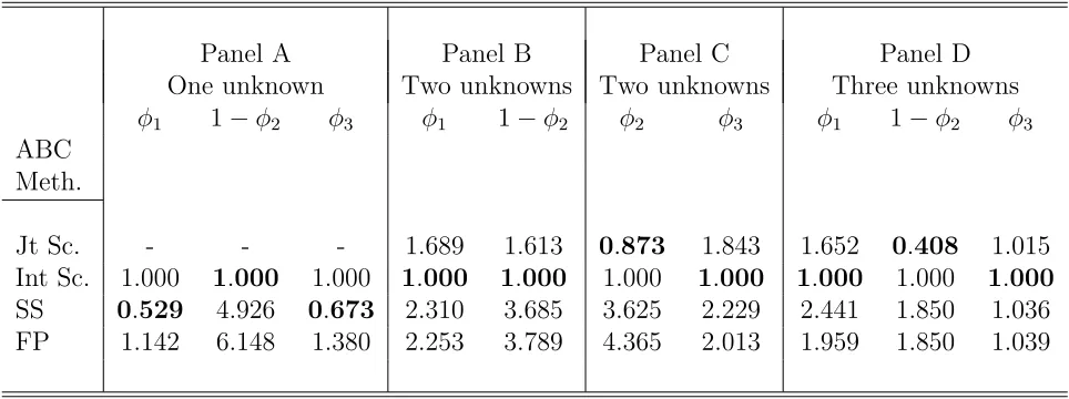
In order to abstract initially from the impact of dimensionality on the ABC methods,
we report results in Panel A for each single parameter of the SV-SQ model, keeping the
remaining two parameters fixed at their true values. In this case the auxiliary-likelihood
method is based on the scalar score statistic, but the RMSE results are recorded in the
row headed ‘Int score’. As is clear, for 1 −φ2 the auxiliary score-based ABC method
produces the most accurate estimate of the exact posterior of all comparators. In the
case of φ1 and φ3 the summary statistic method (based on the Euclidean distance) yields
the most accurate estimate, with the dimension reduction technique of Fearnhead and Prangle (2012) producing the least accurate posterior estimates for both parameters. The
results recorded in Panels B to D highlight that when either two or three parameters are
unknown the score-based ABC method produces the most accurate density estimates in all
cases, with the integrated likelihood technique described in Section 5.1.2 yielding further
accuracy improvements over the joint score (‘Jt Sc.’) methods in five out of the seven
cases, auguring quite well for this particular approach to dimension reduction.
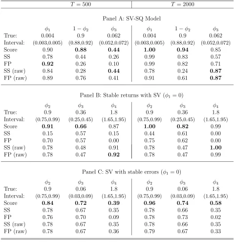
5.2
Large sample performance
5.2.1 Data generation and computational details
For all three examples outlined in Section 4 we now document numerically the extent to
which the auxiliary likelihood-based ABC posteriors become increasingly concentrated (or otherwise) around the true parameters as the sample size increases. To this end, in Table
2 we report the average probability mass (over 50 runs of ABC) within a small interval
around the true parameter, for T = 500 and 2000. Artificial ‘empirical’ data is generated
from the SV-SQ model using the same parameter settings as detailed in Section 5.1.1.
Generation from the other two models uses parameter settings that also yield empirically
plausible data. Once again, as a means of comparison, summary statistic-based results are
Table 1: Average RMSE of an estimated marginal posterior over 50 runs of ABC (each run using 50,000 replications, with 500 draws (1%) retained); recorded as a ratio to the
(average) RMSE for the (integrated) ABC score method. ‘Sc.’ refers to the ABC method based on the score of the AUKF model; ‘SS’ refers to the ABC method based on a Euclidean distance for the summary statistics in (28); ‘FP’ refers to the Fearnhead and Prangle ABC method, based on the summary statistics in (28). For the single parameter case, the (single) score method is documented in the row denoted by ‘Int Sc.’, whilst in
the multi-parameter case, there are results for both the joint (Jt) and integrated (Int) score methods. The bolded figure indicates the approximate posterior that is the most
accurate in any particular instance. The sample size is T = 500.
Panel A Panel B Panel C Panel D
One unknown Two unknowns Two unknowns Three unknowns
φ1 1−φ2 φ3 φ1 1−φ2 φ2 φ3 φ1 1−φ2 φ3
ABC Meth.
Jt Sc. - - - 1.689 1.613 0.873 1.843 1.652 0.408 1.015
Int Sc. 1.000 1.000 1.000 1.000 1.000 1.000 1.000 1.000 1.000 1.000
SS 0.529 4.926 0.673 2.310 3.685 3.625 2.229 2.441 1.850 1.036
FP 1.142 6.148 1.380 2.253 3.789 4.365 2.013 1.959 1.850 1.039
(2012) distance in (30). In order to highlight the dependence of posterior concentration on
the particular choice of summaries, we define the statistics in (28) using both yt = ln(rt2)
andyt=rt, with results for the latter choice recorded in the rows denoted by SS (raw) and
FP (raw). All relevant probabilities are estimated via rectangular integration of the ABC
kernel density ordinates, with the boundaries of the interval used for a given parameter (recorded at the top of the table) determined by the grid used to numerically estimate the
kernel density.
In order to reduce the computational burden, for the SV-SQ model we compute all
probabilities for the (three) single unknown parameter cases only, and as based on 50,000
replications within each of the 50 ABC runs. For the other two models however, since
the auxiliary models employed for both examples feature likelihood functions that are
computationally simple, all parameters are estimated jointly. For both examples, we fix
φ1 = 0, leaving three free parameters, φ2 to φ4. Further, as guided by the theoretical
results in Frazier et al. (2016), for these two models the quantile used to select draws
is allowed to decline as T increases. With 250 draws retained for the purpose of density estimation this means that 55,902 and 447,214 replications (for each of the 50 draws) are