Minimum density hyperplanes in the feature space

Minimum Density Hyperplanes in the Feature Space

Katie R. Yates STOR-i CDT Lancaster University Lancaster, UK, LA1 4YF Email: [email protected]

Nicos G. Pavlidis

Department of Management Science Lancaster University Lancaster, UK, LA1 4YX Email: [email protected]

Abstract—We introduce a kernel formulation of the recently proposed minimum density hyperplane approach to clustering. This enables the identification of clusters that are not linearly separable in the input space by mapping them into a feature space. This mapping also extends the applicability of the minimum density hyperplane to datasets whose features are not necessarily continuous. The location of minimum den-sity hyperplanes involves the optimisation of a non-convex objective function. In the feature space, the dimensionality of the optimisation problem is n, where n is the number of observations. We further propose an approximation method that can substantially reduce the dimensionality of the search space, avoiding searching over dimensions which are unlikely to contain useful information for clustering. Experimental results suggest that the proposed approach is capable of producing high quality partitions across a number of benchmark datasets.

1. Introduction

Given a set of observations, the clustering problem is to partition these into a number of groups, orclusters, so that observations assigned to the same cluster are more similar to each other than observations assigned to different clusters. As there is no unique definition of what constitutes a cluster a number of different approaches have been proposed in the literature, each relying on a different cluster definition. In the nonparametric statistical approach to clustering, also known as density clustering, clusters are defined as contiguous re-gions of high-probability density [1, 2]. Rather than search-ing for dense regions directly, an equivalent formulation is to define cluster boundaries as passing through regions of low probability density; known as low-density separation [3]. The minimum density hyperplane (MDH) [4] is the first approach for the partition of unlabelled or partially labelled data, that directly minimises the integral of the empirical density along a hyperplane separator. This can be done with only the one-dimensional projections onto the normal vec-tor to the hyperplane, making this formulation particularly relevant for high-dimensional problems.

This approach is linked to density clustering as it can be shown that under specific conditions the integral of the empirical density along a hyperplane imposes an

up-per bound on the maximum value of the density at any point along this hyperplane. Therefore, by minimising the integral of the density along the hyperplane separator, the smallest upper bound on the value of the empirical density on the separator is achieved. Low-density separators also play a significant role is the analysis of clustering stability. A close relationship between the stability of a clustering and the data density along the cluster boundaries has been established in [5, 6]. Roughly speaking, the lower these densities the more stable the clustering. The detection of MDHs is also relevant in semi-supervised classification [3], where unlabelled data are used in conjunction with labelled data to improve classification performance compared to just using the (scarce) labelled data. A necessary assumption for this to be feasible is that a better knowledge of the probability distribution of the observed data,p(x)improves the inference of the class-conditional densitiesp(x|y), where ydenotes the classification label. A standard assumption of this type, underlying popular methods like the transductive support vector machine [7], is that class boundaries pass through regions of low probability density.

An important restriction of the MDH approach is that it cannot correctly identify clusters that are not linearly separable. In this work we propose the kernel MDH to overcome this limitation. We first map the data nonlinearly into a feature space and a MDH is sought in the new feature space. The hyperplane separator in the feature space corresponds to a nonlinear separator in the input space. The potentially high dimensionality of the feature space means it is not feasible to calculate the mapped observations (feature vectors) explicitely. However, their one-dimensional projec-tions onto any vector in the feature space may be calculated using the matrix of pairwise inner products (kernel matrix). This is sufficient to allow the location of the MDH in the feature space.

of the feature space.

The remaining paper is organised as follows: Section 2 presents the formulation of the MDH in feature space and the approximation in a subspace. Section 3 provides an em-pirical evaluation of the binary partitions from the proposed approach and alternative established kernel based clustering algorithms across benchmark datasets with varying charac-teristics. Conclusions are discussed in Section 4.

2. Minimum Density Hyperplanes

We assume a finite set of observations,S ={xi}ni=1⊂

X, where X denotes the input space. A hyperplane is parameterised by its normal vector,v∈Xand displacement from the origin b ∈ _R, H(v, b) = {x∈X| hv,xi=b}. Without loss of generality [4] restrict attention tokvk2= 1. The density on H(v, b), as defined by [8], is given by the integral of the density functionpalong the hyperplane,

I(v, b) = Z

H(v,b)

p(x)dx. (1)

In all practical applications the density function p is un-known. In the original MDH approach [4] a continuous density estimator with isotropic Gaussian kernels is used. The advantage of this is that ifX⊂Rd then the estimated

density on a hyperplane, Iˆ(v, b) can be evaluated exactly from one-dimensional projections,

ˆ I(v, b) =

Z

H(v,b)

1

n(2πh2₎d 2

n X

i=1

exp

−kx−xik 2

2h2

dx,

= 1

nh√2π n X

i=1

exp

−(b− hv,xii) 2

2h2

. (2)

In detail, Eq. (2) states that Iˆ(v, b) can be evaluated by projecting the data ontov; constructing a one-dimensional kernel density estimator with the same bandwidth param-eter h; and evaluating it at b. Since the above equation requires only the evaluation of the inner product between the projection vector,v, and the observations, xi, it can be generalised to a kernel-defined feature space.

Letκ(x,z) be a kernel and φ:X→F a feature map satisfyingκ(x,z) =hφ(x), φ(z)iF. Although in the general case it might not be possible to define the projection vector in the feature space, the representer theorem [9] allowsvto be expressed in its dual representation,v=Pn_i=1αiφ(xi). With this representation and restricting attention to {v ∈

F|kvkF = 1}, the projection of the feature vector, φ(xj) ontovis given by,

hφ(xj),viF=

Pn

i=1αiKi,j

(α>_Kα)1/2, (3) whereα∈Rn, andK∈Rn×n is the kernel matrix whose

entries areKij =κ(xi,xj). The density on a hyperplane in the feature space is therefore,

ˆ

I(α, b) = 1 nh√2π

n X

j=1

exp (

−(b− hφ(xj),viF) 2

2h2

) , (4)

where use use the notationIˆ(α, b)to stress the fact that we rely on the dual representation ofv. [10] show that learning

αis equivalent to learningv. Practically, this results in the seach space for the MDH beingn-dimensional.

We denote the kernel minimum density hyperplane (KMDH) to be the hyperplane H(α?, b?) that min-imises Iˆ(α, b). with the induced partition being Π1 = {xj|hφ(xj),viF > b?}, Π2 = {xj|hφ(xj),viF 6 b?}. Arbitrarily small values ofIˆ(α, b)can be trivially obtained by allowing |b| → ∞. Clearly such hyperplanes are not meaningful for clustering as they assign all points to one partition. To avoid such situations it is necessary to constrain the range ofb. If we assume without loss of generality that the mean of all the feature vectors is zero, then one can constrainbto be in an interval around the standard deviation of the projected data,b∈[−γσα, γσα].

ˆ

I(α, b)can be optimised using constrained optimisation methods but this approach has been shown to be highly susceptible to convergence to local minima. To prevent this, [4] propose a projection pursuit formulation where the constraints on bare imposed through a penalty function. In this formulation the objective function, θ, is defined as,

θ(α) = min b∈R

f(α, b), (5)

f(α, b) = ˆI(α, b) + L

ηmax{0,−γσα−b, b−γσα} 1+

(6)

where L = (e1/2_h2_2π)−1_{, ∈ (0,1) and η ∈ (0,1).} The above settings ensure that the minimiser of f(α, b) is within η of the minimiser of Iˆ(α, b). By optimising θ(α)

instead of Iˆ(α, b)this approach can accomodate discontin-uous changes in the location of the minimiser of the one-dimensional kernel density estimator, Iˆ(α, b) with respect to changes in α. This comes at the cost of rendering the objective function non-smooth for values of α for which argminb∈Rf(α, b) is not a singleton. Although standard

gradient descent methods are not guaranteed to converge for non-smooth functions, [11] have strongly advocated that a simple BFGS method with inexact line searches is very efficient in practice. We therefore use BFGS in our experiments.

2.1. Computational Complexity

In this subsection, we discuss the computational com-plexity of KMDH. At each iteration, the algorithm projects the data onto v, at a cost of O(n(n+ 1)). Then, to obtain the projection index θ(α), it is necessary to minimise the penalised objective f(α, b). This minimisation is possible by evaluating f(α, b) on a grid ofm points, involving m evaluations of a density estimate with n components. The cost of this may be reduced from O(mn) to O(n+m)

advocated by [11, 4]. This can be done at a cost ofO(n2_)per iteration [13, Pg. 140] plus the cost of function evaluations off(α, b)as defined as above and gradient evaluations with costO(n(n+ 1)).

2.2. Approximation methods - Subspace

Since the normal vector to the hyperplanevis expressed by its dual vectorα∈Rn, the search space for the KMDH

isn-dimensional. However, whennis large, the optimisation is computationally expensive and it is likely that a number of these dimensions are not necessary to locate a low density separator. Hence, we consider using only a subspace ofFto search for the minimum density hyperplane. We use kernel principal component analysis (KPCA) [14] to reduce the dimensionality of the search space while retaining maximal variability. Although there is no guarantee that directions of high variability will be meaningful for cluster detection [15, 4] it is arguably unlikely that directions which exhibit almost no variability are relevant for clustering. We denote this subspaceF0⊆Rn

0

wheren0 n. LetU∈Rn×n

0

= (u1, ...,un0)be the matrix of the dual

vectors of the first n0 unit principal component vectors of

Fas columns. InF0, the matrix of pairwise inner products of the feature vectors is K0 = U>KU ∈ Rn

0_×n0

. Then, the projection of the feature vectorφ(xj)onto the vectorv whose dual vector isβ=Pn

0

i=1α0iu>i ∈R n _is,

hφ(xj),viF0 =

Pn0

i=1α0iKi,j0

(α0>_K0_α0₎1/2. (7)

This results in a search over the n0 _{dimensions of the} subspace defined by U. This approach is equivalent to calculating the projections of the feature vectors onto the first n0 kernal principal components and then locating the MDH as in [4].

We then seek the α0? andb? which minimise

θ(α0) = min b∈R

f(α0, b), (8)

f(α0, b) = ˆI(α0, b) + L

ηmax{0,−γσα0−b, b−γσα0} 1+_,

(9)

ˆ

I(α0, b) = 1 nh√2π

n X

j=1

exp (

−(b− hφ(xj),viF0) 2

2h2

)

(10)

where σα0 is the standard deviation of the projections

defined by Eq. 7. The subspace kernel minimum density hyperplane (S-KMDH) is then the hyperplane H(α0?_{, b}?₎ that minimises f(α0, b). This induces the partition Π1 = {xj|hφ(xj),viF0 > b?}, Π₂ = {x_j|hφ(x_j),vi_F0 6 b?}.

The smaller dimensionality ofF0 _{reduces the computational} cost of calculating the projections and the gradient evalua-tions toO(n0(n0+1))and avoids searching over dimensions which are potentially not useful for cluster detection.

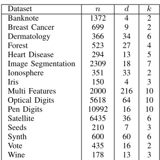
TABLE 1. SUMMARY OFUCIBENCHMARK DATASETS.

Dataset n d k

Banknote 1372 4 2

Breast Cancer 699 9 2

Dermatology 366 34 6

Forest 523 27 4

Heart Disease 294 13 5

Image Segmentation 2309 18 7

Ionosphere 351 33 2

Iris 150 4 3

Multi Features 2000 216 10

Optical Digits 5618 64 10

Pen Digits 10992 16 10

Satellite 6435 36 6

Seeds 210 7 3

Synth 600 60 6

Vote 435 16 2

Wine 178 13 3

3. Experimental Results

In this section, we conduct an empirical evaluation of the proposed approaches, KMDH and S-KMDH. We com-pare the quality of the binary partitions produced by these approaches to kernel k-means [16] and spectral clustering [17] across a variety of benchmark datasets from the UCI repository [18]. The main characteristics of these datasets are summarised in Table 1 where n, d and k correspond to the number of observations, dimensions and clusters respectively.

3.1. Measuring the Quality of Binary Partitions

Since we are looking for binary partitions of datasets which may contain an arbitrary number of clusters, we use the two performance measures outlined in [4]. Both take values in the range

[0,1]with larger values indicating a higher quality partition. It is

assumed that a desirable partition into two groups, Π1 and Π2

should both avoid the division of clusters between elements of the partition and separate at least one cluster from the remaining data. This is captured by the modification of the true cluster labels to reflect the partition to which the majority of the elements of each cluster are assigned. In the case of equal numbers of observations from a cluster being assigned to each partition, the cluster is assigned to the smaller partition. The true cluster labels are then

merged into two aggregate clustersC1 andC2.

The success ratio (SR) of a partition requires both the error

and success of a partition, denoted E(Π1,Π2) and S(Π1,Π2)

respectively. The success (error) of a binary partition is defined as the number of elements belonging to the same aggregate cluster

which are (are not) assigned to the same partition. The SR ofΠ1,

Π2measures the extent to which the majority of at least one cluster

is distinguished from the rest of the data,

S(Π1,Π2) = min{max{|Π1∩C1|,|Π1∩C2|}, (11)

max{|Π2∩C1|,|Π2∩C2|}}, E(Π1,Π2) = min{|Π1∩C1|+|Π2∩C2|, (12)

|Π1∩C2|+|Π2∩C1|},

SR(Π1,Π2) =

S(Π1,Π2) S(Π1,Π2) +E(Π1,Π2)

. (13)

The second measure is the binary V-measure (VM). This is

(a) Initialisation (b)γ=10−3 _{(c)γ= 0.5}

Figure 1. Visualisation of KMDH on Synth dataset.

C2. The V-measure measures the properties of both homogeneity

and completeness. The former measures the conditional entropy of the aggregate cluster distribution within each partition. The latter measures the conditional entropy of the partition within each aggregate cluster. The V-measure is calculated as the weighted harmonic mean of homogeneity and completeness. Both SR and VM return a value of zero if an algorithm fails to distinguish the majority of any cluster from the rest of the data. This is not necessarily the case for alternative metrics [4].

3.2. Details of Implementation

As for all kernel-based approaches, the choice of kernel func-tion impacts greatly on the results produced. In the absence of prior knowledge to guide the choice of kernel, we use the radial basis (RBF) kernel function

Kij=κ(xi,xj) = exp

−||xi−xj|| 2

2σ2

. (14)

This is the most widely used kernel in the literature.

The parameters which can strongly influence the result of our

approach are the bandwidth of the density estimate, h and the

interval width,γ. We useh= 0.9ˆσn−1/5

whereσˆis the standard

deviation of the projections of the feature vectors as defined by Eqs. (3) and (7) for KMDH and S-KMDH respectively. This is the recommended bandwidth selection rule when the density is

assumed to be multimodal [20]. The interval width parameter γ

is initialised close to zero, inducing a balanced partition. This is

gradually increased to γmax = 0.9 to allow convergence to the

minimum integrated density [4].

Although generally robust to convergence to poor local min-ima, the results produced by KMDH can depend upon initialisa-tion. We tried initialising on the kernel principal components and random vectors. Generally, the first kernel principal component led to the best partitions however, we also present results based on ten random initialisations as a comparison. In S-KMDH, we experimented with principal component and random initialisa-tions. As for KMDH, the best results were generally produced by initialising on the first principal component, hence these are

presented. For the choice of dimensionality of the subspacen0, we

used the eigenvalues from KPCA to select the dimensionality that

retained 90% of the variability. Where necessary, we present the

performance of the partition based on the sutability of the resulting projections onto the normal vector to the hyperplane for clustering. For this we consider the structure in the estimated density of the projections [21, 4]. In this paper we use the relative depth of the estimated density of the one-dimensional projections,

RelativeDepth(v) =min{pˆv(ml),pˆv(mr)} −pˆv(b ?₎

ˆ

pv(b?)

(15)

wherevis an arbitrary projection vector whose projected feature

vectors have estimated densitypˆvandmlandmrare the locations

of the modes to the left and right of b? inpˆv respectively. This

●● ● ●

●

● ●

●

● ●

●

● ●

● ● ●

●

●●

● ●

● ●

0.00 0.25 0.50 0.75

KMDH_PCA KMDH_Rand S

−_KMDH K−_k −means

Spectr

al

Method

Regret

Measure

SR VM

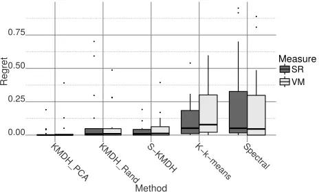
Figure 2. Box plot of regret with respect to SR and VM across UCI benchmark datasets.

criterion favours projection directions with low minima between two modes. In our experience, this criterion is better than just using the value of the integrated density which can lead to separators which do not actually separate the data.

For the comparison to kernelk-means and spectral clustering,

we used the implementation in the kernlab package for R [22] with the same kernel matrix as for our algorithms.

3.3. Visualisation

An attractive property of locating partitions based on one-dimensional projections only is the ability to plot the iterations of the algorithm, allowing interpretable visualisations of the resulting partitions. Figure 1 illustrates iterations of KMDH on the Synth dataset. The estimated density of the projections, the penalised

objective f(α, b) and the current split point are indicated by

black solid, blue dashed and red dotted lines respectively. The projected feature vectors are plotted as points whose colours and markers correspond to the true cluster labels. These are separated

along they-axis for illustration purposes. Figure 1(a), shows that

the estimated density of the initial projections does not have a

strong bi-modal structure. Here, the minimum off(α, b)is quite

high and the associated separating hyperplane cannot partition the

clusters. Figure 1(b) shows that optimisingαover a small range

forblocates a hyperplane with a much lower integrated density.

This induces a balanced partition between two clear modes of the estimated density of the projections. Finally, Figure 1(c) shows

that increasing the width of the search interval forb, allows the

location of the hyperplane which minimises the integrated density and does not intersect the true clusters.

3.4. Performance Evaluation

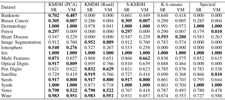
In this section, we present the performance of our proposed methods across the 16 UCI benchmark datasets summarised in Table 1. Table 2 reports the SR and VM scores for KMDH (with

KPCA and random initialisations), S-KMDH (withn0 set to retain

90% of the variability), kernel k-means and spectral clustering.

The best performing method for each dataset is indicated in bold font. Across all datasets, KMDH and S-KMDH perform

consis-tently well and frequently perform better than kernel k-means

and spectral clustering. Generally, the performance of S-KMDH is competitive with KMDH achieving close to the same performance

on almost all datasets. For largen, the search space for KMDH is

TABLE 2. SRANDVMSCORES OF BINARY PARTITIONS FROMKMDH, S-KMDH,KERNELk-MEANS AND SPECTRAL CLUSTERING ONUCI

BENCHMARK DATASETS. BOLD FONT INDICATES THE BEST PERFORMANCE FOR EACH DATASET.

Dataset KMDH (PCA) KMDH (Rand) S-KMDH K-k-means Spectral

SR VM SR VM SR VM SR VM SR VM

Banknote 0.702 0.487 0.000 0.000 0.661 0.449 0.640 0.418 0.000 0.000

Breast Cancer 0.305 0.007 0.286 0.004 0.305 0.007 0.290 0.005 0.285 0.004

Dermatology 1.000 1.000 0.978 0.941 1.000 1.000 0.991 0.973 1.000 1.000

Forest 0.297 0.009 0.000 0.000 0.297 0.009 0.290 0.007 0.179 0.010

Heart Disease 0.547 0.229 0.000 0.000 0.547 0.229 0.593 0.280 0.583 0.263

Image Segmentation 0.912 0.760 0.952 0.889 0.912 0.760 0.783 0.574 0.000 0.000

Ionosphere 0.540 0.276 0.527 0.267 0.533 0.258 0.000 0.000 0.000 0.000

Iris 1.000 1.000 1.000 1.000 1.000 1.000 1.000 1.000 1.000 1.000

Multi Features 0.871 0.657 0.868 0.651 0.866 0.662 0.838 0.575 0.852 0.615

Optical Digits 0.917 0.809 0.895 0.766 0.810 0.639 0.688 0.464 0.000 0.000

Pen Digits 0.821 0.622 0.832 0.629 0.821 0.623 0.785 0.576 0.783 0.538

Satellite 0.729 0.419 0.919 0.766 0.727 0.416 0.690 0.368 0.866 0.810

Seeds 0.917 0.800 0.917 0.800 0.917 0.800 0.861 0.703 0.795 0.644

Synth 1.000 1.000 0.873 0.718 1.000 1.000 0.863 0.704 1.000 1.000

Votes 0.798 0.522 0.798 0.522 0.767 0.418 0.787 0.493 0.780 0.478

Wine 0.983 0.951 0.983 0.951 0.931 0.857 0.674 0.353 0.727 0.588

datasets, the computational advantage of using a reduced search

space is less apparent, hence searching over allndimensions may

be feasible to achieve better performance.

The results from the random initialisations of KMDH indicate that the quality of the partition produced depends on the initial projection direction. This is particularly evident for the Banknote dataset where random initialisations completely fail to correctly identify any clusters. Often, initialising on the first kernel principal component produces the best partitions and avoids the computa-tional cost of running multiple random initialisations to achieve a competitive result.

Figure 2 provides box plots of the regret of an algorithm across these datasets with respect to SR and VM. The regret of an algorithm refers to the difference between its performance and that of the best performing algorithm. Therefore, a regret close to zero indicates consistently high quality partitions relative to other algorithms. KMDH initialised on the first kernel principal component minimises the regret across these datasets. KMDH with random initialisation is also competitive with this while S-KMDH has the third lowest regret. This suggests that the minimum density hyperplane approach frequently locates better partitions

than spectral clustering or kernel k-means. For large datasets,

the reduced computational cost of S-KMDH while maintaining a competitive performance makes this a desirable approximation technique.

4. Conclusion

We introduced an approach to locate minimum density hyper-plane separators for data which are not linearly separable in the input space. This is done by mapping the set of observations into a feature space by a nonlinear kernel function. Hyperplane separators in this feature space then correspond to nonlinear separators in the input space. The density intersected by a linear separator can be evaluated using the estimated density of the one-dimensional projections of the feature vectors onto the vector normal to the hyperplane. The calculation of these projections can be done using the kernel matrix of the pairwise inner products of the feature vectors only. The location of the MDH in the feature space requires

the solution of an n-dimensional optimisation problem with a

computational costO(n(n+ 1)).

In many practically interesting problems,nis large, in which

case it is not feasible or necessary to search over allndimensions

of the search space to locate low density separators. Hence, we propose an approximation method which uses a lower-dimensional subspace of the feature space to search for a low density separating hyperplane. This aims to avoid searching over dimensions which do not contain meaningful information for clustering.

We undertook an empirical evaluation of the performance of our approaches across a variety of UCI benchmark datasets.

This showed that optimising over the full n-dimensional search

space for the minimum density hyperplane produced the best par-titions. However, in the majority of cases, using significantly fewer dimensions produced similar or equivalent results at a reduced computational cost. This is particularly useful for large datasets where the significant reduction in computational cost may out weigh the small reduction in the quality of the partition. Using random initialisations indicate that the partitions produced by our approaches can be sensitive to initialisation for some datasets and we recommend initialising on the first principal component. Overall, our results show that our algorithms produce consistently high quality binary partitions, performing better or equivalent to

kernelk-means and spectral clustering in almost all cases.

References

[1] A. Azzalini and N. Torelli, “Clustering via nonparametric density estimation,”Statistics and Computing, vol. 17, no. 1, pp. 71–80, 2007.

[2] W. Stuetzle and R. Nugent, “A generalized single linkage method for estimating the cluster tree of a density,”Journal of Computational and Graphical Statistics, vol. 19, no. 2, pp. 397–418, 2010.

[3] O. Chapelle, B. Sch¨olkopf, and A. Zien,Semi-Supervised Learning, ser. Adaptive computation and machine learning. MIT Press, 2006.

[4] N. Pavlidis, D. Hofmeyr, and S. Tasoulis, “Minimum density hyper-planes,”Journal of Macnine Learning Research (forthcoming), 2016.

[5] S. Ben-David and U. von Luxburg, “Relating clustering stability to properties of cluster boundaries,” inProceedings of the Conference on Learning Theory (COLT), 2008, pp. 379–390.

[6] O. Shamir and N. Tishby, “Model selection and stability in k -means clustering,” in Proceedings of the Conference on Learning Theory (COLT), 2008, pp. 367–378.

[8] S. Ben-David, T. Lu, D. P´al, and M. Sot´akov´a, “Learning low-density separators,” inProceedings of the 12th International Conference on Artificial Intelligence and Statistics (AISTATS), ser. JMLR Workshop and Conference Proceedings, D. van Dyk and M. Welling, Eds., Florida, USA, 2009, pp. 25–32.

[9] B. Sch¨olkopf, R. Herbrich, and A. J. Smola, “A generalized represen-ter theorem,” inInternational Conference on Computational Learning Theory. Springer, 2001, pp. 416–426.

[10] J. Shawe-Taylor and N. Cristianini,Kernel methods for pattern anal-ysis. Cambridge university press, 2004.

[11] A. Lewis and M. Overton, “Nonsmooth optimization via quasi-Newton methods,” Mathematical Programming, vol. 141, pp. 135– 163, 2013.

[12] V. I. Morariu, B. V. Srinivasan, V. C. Raykar, R. Duraiswami, and L. S. Davis, “Automatic online tuning for fast gaussian summation,” in Advances in Neural Information Processing Systems, 2009, pp. 1113–1120.

[13] J. Nocedal and S. Wright,Numerical Optimization. Springer Science & Business Media, 2006.

[14] B. Sch¨olkopf, A. Smola, and K.-R. M¨uller, “Kernel principal com-ponent analysis,” in International Conference on Artificial Neural Networks. Springer, 1997, pp. 583–588.

[15] H.-P. Kriegel, P. Kr¨oger, and A. Zimek, “Clustering high-dimensional data: A survey on subspace clustering, pattern-based clustering, and correlation clustering,”ACM Transactions on Knowledge Discovery from Data (TKDD), vol. 3, no. 1, p. 1, 2009.

[16] R. Zhang and A. I. Rudnicky, “A large scale clustering scheme for kernel k-means,” in Pattern Recognition, 2002. Proceedings. 16th International Conference on, vol. 4. IEEE, 2002, pp. 289–292.

[17] U. Von Luxburg, “A tutorial on spectral clustering,” Statistics and Computing, vol. 17, pp. 395 – 416, 2007.

[18] M. Lichman, “UCI machine learning repository,” 2013. [Online]. Available: http://archive.ics.uci.edu/ml

[19] A. Rosenberg and J. Hirschberg, “V-measure: A conditional entropy-based external cluster evaluation measure.” inEMNLP-CoNLL, vol. 7. Citeseer, 2007, pp. 410–420.

[20] B. W. Silverman,Density estimation for statistics and data analysis. CRC press, 1986, vol. 26.

[21] S. K. Tasoulis, M. G. Epitropakis, V. P. Plagianakos, and D. K. Tasoulis, “Density based projection pursuit clustering,” in2012 IEEE Congress on Evolutionary Computation. IEEE, 2012, pp. 1–8.